Phase Portraits of Complex Functions - the R Package viscomplexr

Peter Biber

Introduction

The R package viscomplexr has been written as a visualization tool for complex functions. More precisely, it provides functionality for making phase portraits of such functions. The method, sometimes called domain coloring, exists in many sub-varieties. However, from the author’s point of view, the style proposed by E. Wegert in his book Visual Complex Functions (Wegert 2012) comes with a particular clarity and a special aesthetic appeal at the same time. Therefore, this package closely follows Wegert’s conventions. Conceptually, the package is intended for being used inside the framework of R’s base graphics, i.e. users of this package can freely utilize all features of base graphics for obtaining an optimum result, be it for scientific or artistic purposes. This article is not at all an introduction to function theory or an exhaustive treatment of what can be done with phase portraits - I recommend Wegert’s book for an ideal combination of both; the purpose of this article is in fact to make the reader acquainted with the technical features the package provides in a step-by-step process.

While the text of this article is virtually identical with the package’s vignette as available on CRAN, CRAN’s size restrictions do not apply here. Therefore, you will find considerably more illustrations below.

Using the function phasePortrait

Visualizing the complex plane

The package does not contain many functions, but provides a very versatile workhorse called phasePortrait. We will explore some of its key features now. Let us first consider a function that maps a complex number \(z \in \mathbb{C}\) on itself, i.e. \(f(z)=z\). After attaching the package with library(viscomplexr), a phase portrait of this function is obtained very easily with:

phasePortrait("z", xlim = c(-8.5, 8.5), ylim = c(-8.5, 8.5),
              xlab = "real", ylab = "imaginary", main = "f(z) = z")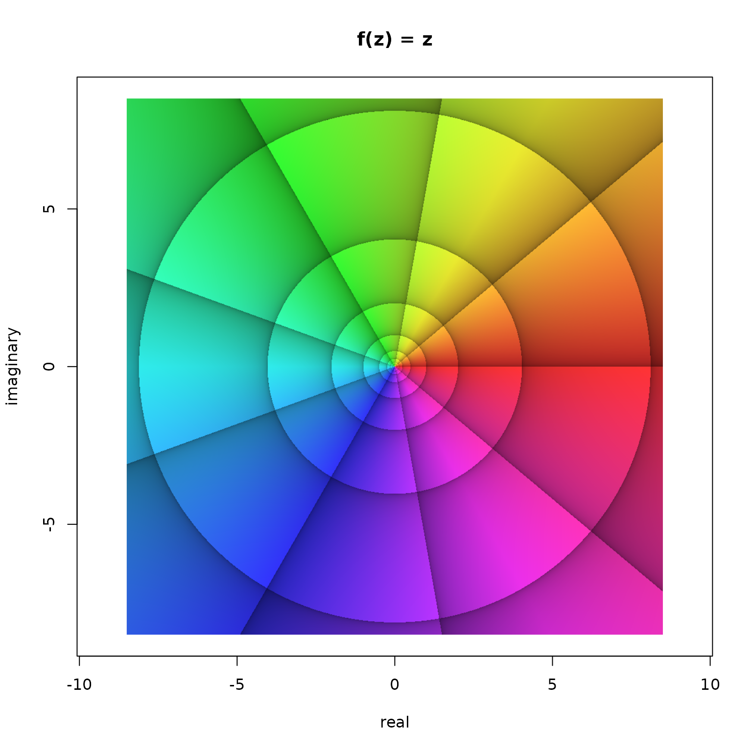

Phase portrait of the function \(f(z)=z\) in the window \(\left|\Re(z)\right| < 8.5\) and \(\left|\Im(z)\right| < 8.5\).

Such a phase portrait is based on the polar representation of complex numbers. Any complex number \(z\) can be written as \(z=r\cdot\mathrm{e}^{\mathrm{i}\varphi}\) or equivalently \(z=r\cdot(\cos\varphi+\mathrm{i}\cdot\sin\varphi)\), whereby \(r\) is the modulus and the angle \(\varphi\) is the argument. The argument, also called the phase angle, is the angle in the origin of the complex number plane between the real axis and the position vector of the number in counter-clockwise orientation. The main feature of a phase portrait is to translate the argument into a color. In addition, there are options for visualizing the modulus or, more precisely, its relative change.

The translation of the phase angle \(\varphi\) into a color follows the hsv color model, where radian values of \(\varphi=0+k\cdot2\pi\), \(\varphi=\frac{2\pi}{3}+k\cdot2\pi\), and \(\varphi=\frac{4\pi}{3}+k\cdot2\pi\) with \(k\in\mathbb{Z}\) translate into the colors red, green, and blue, respectively, with a continuous transition of colors with values between. As all numbers with the same argument \(\varphi\) obtain the same color, the numbers of the complex plane as visualized in the Figure above are colored along the chromatic cycle. In order to add visual structure, argument values of \(\varphi=\frac{2\pi}{9}\), i.e. \(40°\) and their integer multiples are emphasized by black lines. Note that each of these lines follows exactly one color. Moreover, the zones between two neighboring arguments \(\varphi_1=k\cdot\frac{2\pi}{9}\) and \(\varphi_2=(k+1)\cdot\frac{2\pi}{9}\) with \(k\in\mathbb{Z}\) are shaded in a way that the brightness of the colors inside one such zone increases with increasing \(\varphi\), i.e. in counterclockwise sense of rotation.

The other lines visible in the figure above relate to the modulus \(r\). One such line follows the same value of \(r\); it is thus obvious that each of these iso-modulus lines must form a concentric circle on the complex number plane (see the figure above). The distance between neighboring iso-modulus lines is chosen so that it always indicates the same relative change. For reasons to talk about later (see also Wegert 2012), the default setting of the function phasePortrait is a relative change of \(b=\mathrm{e}^{2\pi/9}\) which is very close to \(2\). Thus, with a grain of salt, the modulus of the complex numbers doubles or halves when moving from one iso-modulus line to the other. In the phase portrait, the zones between two adjacent iso-modulus lines are shaded in a way that the colors inside such a zone become brighter in the direction of increasing modulus. The lines themselves are located at the moduli \(r=b^k\), with \(k\in\mathbb{Z}\). This is nicely visible in the phase portrait above, where the outmost circular iso-modulus line indicates (approximately, as \(b\) is not exactly \(2\)) \(r=2^3=8\). Moving inwards, the following iso-modulus lines are at (approximately) \(r=2^2=4\), \(r=2^1=2\), \(r=2^0=1\), \(r=2^{-1}=\frac{1}{2}\), \(r=2^{-2}=\frac{1}{4}\), etc. Obviously, as the modulus of the numbers on the complex plane is their distance from the origin, the width of the concentric rings formed by adjacent iso-modulus lines approximately doubles from ring to ring when moving outwards.

Visual structuring - the argument pType

When working with the function phasePortrait, it might not always be desirable to display all of these reference lines and zonings. The argument pType allows for four different options as illustrated in the next example:

# divide graphics device into four regions and adjust plot margins 
op <- par(mfrow = c(2, 2), 
          mar   = c(0.25, 0.55, 1.10, 0.25)) 
# plot four phase portraits with different choices of pType
phasePortrait("z", xlim = c(-8.5, 8.5), ylim = c(-8.5, 8.5), pType = "p",
              main = "pType = 'p'",   axes = FALSE)
phasePortrait("z", xlim = c(-8.5, 8.5), ylim = c(-8.5, 8.5), pType = "pa",
              main = "pType = 'pa'",  axes = FALSE)
phasePortrait("z", xlim = c(-8.5, 8.5), ylim = c(-8.5, 8.5), pType = "pm",
              main = "pType = 'pm'",  axes = FALSE)
phasePortrait("z", xlim = c(-8.5, 8.5), ylim = c(-8.5, 8.5), pType = "pma",
              main = "pType = 'pma'", axes = FALSE)
par(op) # reset the graphics parameters to their previous values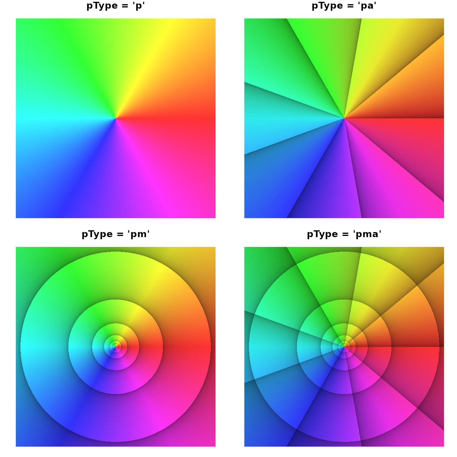

Different options for including reference lines with the argument pType.

As evident from the figure above, setting ptype to ‘p’ displays a phase portrait in the literal sense, i.e. only the phase of the complex numbers is displayed and nothing else. The option ‘pa’ adds reference lines for the argument, the option ‘pm’ adds iso-modulus lines, and the (default) option ‘pma’ adds both. In addition to these options, the example shows phasePortrait in combination with R’s base graphics. The first and the last line of the code chunk set and reset global graphics parameters, and inside the calls to phasePortrait, we use the arguments main (diagram title) and axes which are generic plot arguments.

Visual structuring - the arguments pi2Div and logBase

For demonstrating options to adjust the density of the argument and modulus reference lines, consider the rational function \[ f(z)=\frac{(3+2\mathrm{i}+z)(-5+5\mathrm{i}+z)}{(-2-2\mathrm{i}+z)^2} \] Evidently, this function has two zeroes, \(z_1=-3-2\mathrm{i}\), and \(z_2=5-5\mathrm{i}\). It also has a second order pole at \(z_3=2+2\mathrm{i}\). We make a phase portrait of this function over the same cutout of the complex plane as we did in the figures above. When calling phasePortrait with such simple functions, it is most convenient to define them as as a quoted character string in R syntax containing the variable \(z\). Run the code below for displaying the phase portrait (active 7” x 7” screen graphics device suggested, e.g. x11()).

op <- par(mar = c(5.1, 4.1, 2.1, 2.1), cex = 0.8) # adjust plot margins 
                                                  # and general text size
phasePortrait("(3+2i+z)*(-5+5i+z)/(-2-2i+z)^2", 
              xlim = c(-8.5, 8.5), ylim = c(-8.5, 8.5),
              xlab = "real", ylab = "imaginary")
par(op) # reset the graphics parameters to their previous values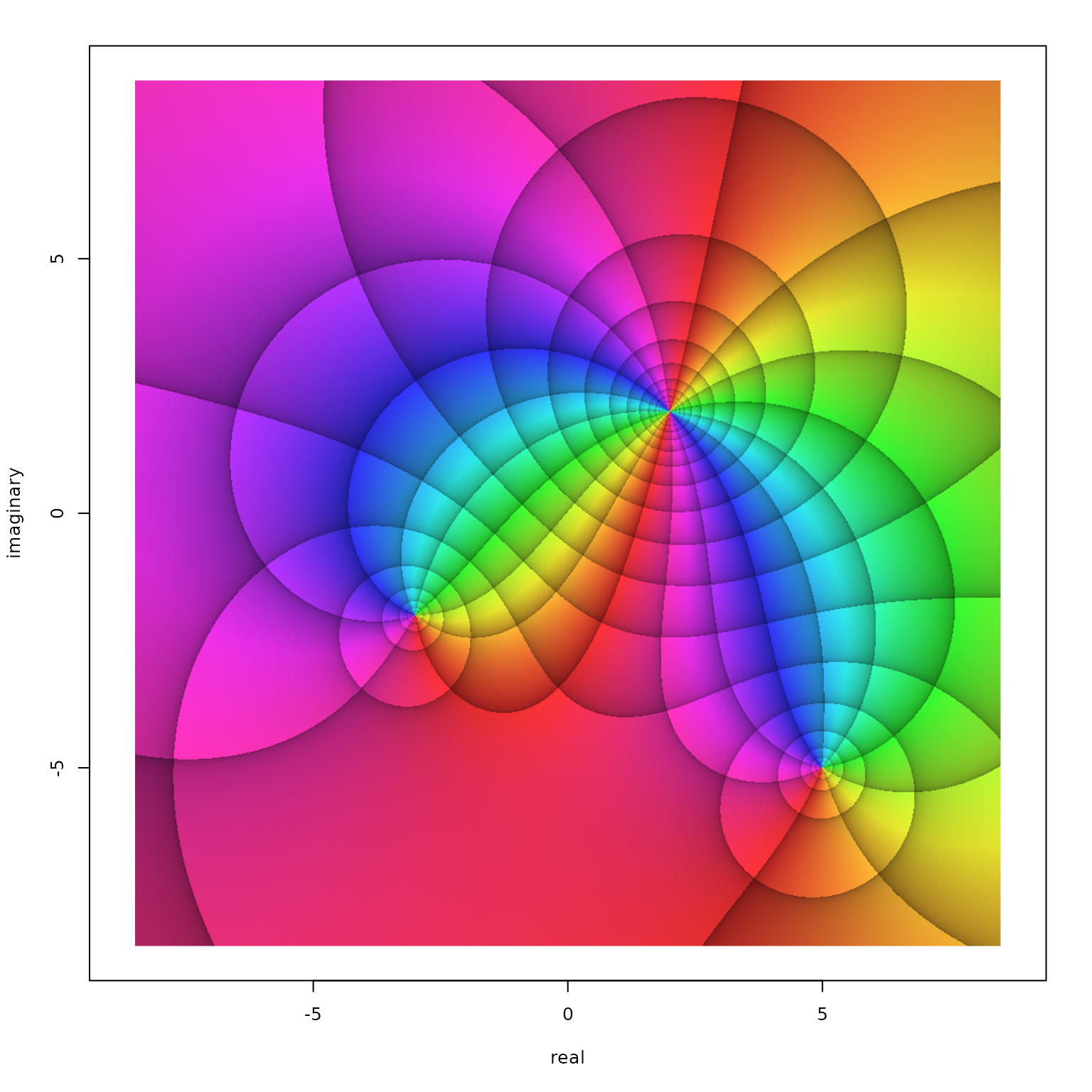

Phase portrait of the function \(f(z)=\frac{(3+2\mathrm{i}+z)(-5+5\mathrm{i}+z)}{(-2-2\mathrm{i}+z)^2}\) in the window \(\left|\Re(z)\right| < 8.5\) and \(\left|\Im(z)\right| < 8.5\).

The resulting figure nicely displays the function’s two zeroes and the pole. Note that all colors meet in zeroes and poles. Around zeroes, the colors cycle counterclockwise in the order red, green, blue, while this order is reversed around poles. For \(n\)^th order (\(n\in\mathbb{N}\)) zeroes and poles, the cycle is passed through \(n\) times. I recommend to check this out with examples of your own.

Now, suppose we want to change the density of the reference lines for the phase angle \(\varphi\). This can be done by way of the argument pi2Div. For usual applications, pi2Div should be a natural number \(n\:(n\in\mathbb{N})\). It defines the angle \(\Delta\varphi\) between two adjacent reference lines as a fraction of the round angle, i.e. \(\Delta\varphi=\frac{2\pi}{n}\). The default value of pi2Div is 9, i.e. \(\Delta\varphi=\frac{2\pi}{9}=40°\). Let’s plot our function in three flavors of pi2Div, namely, 6, 9 (the default), and 18, resulting in \(\Delta\varphi\) values of \(\frac{\pi}{3}=60°\), \(\frac{2\pi}{9}=40°\), and \(\frac{\pi}{9}=20°\). In order to suppress the iso-modulus lines and display the argument reference lines only, we are using pType = "pa".

# divide graphics device into three regions and adjust plot margins 
op <- par(mfrow = c(1, 3), mar = c(0.2, 0.2, 0.4, 0.2))
for(n in c(6, 9, 18)) {
  phasePortrait("(3+2i+z)*(-5+5i+z)/(-2-2i+z)^2", xlim = c(-8.5, 8.5), ylim = c(-8.5, 8.5),
                pi2Div = n, pType = "pa", axes = FALSE)
  # separate title call (R base graphics) for nicer line adjustment, just cosmetics
  title(paste("pi2Div =", n), line = -1.2) 
}
par(op) # reset graphics parameters to previous values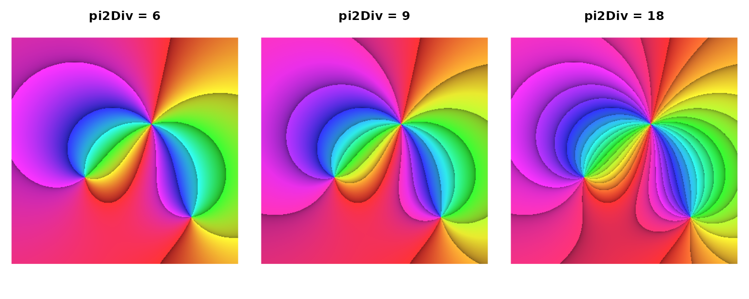

The function \(f(z)=\frac{(3+2\mathrm{i}+z)(-5+5\mathrm{i}+z)}{(-2-2\mathrm{i}+z)^2}\) portrayed with three different settings of pi2Div and pType = "pa".

So far, this is exactly, what had to be expected. But see what happens when we choose the default pType, "pma" which also adds modulus reference lines:

# divide graphics device into three regions and adjust plot margins 
op <- par(mfrow = c(1, 3), mar = c(0.2, 0.2, 0.4, 0.2))
for(n in c(6, 9, 18)) {
  phasePortrait("(3+2i+z)*(-5+5i+z)/(-2-2i+z)^2", xlim = c(-8.5, 8.5), ylim = c(-8.5, 8.5),
                pi2Div = n, pType = "pma", axes = FALSE)
  # separate title call (R base graphics) for nicer line adjustment, just cosmetics
  title(paste("pi2Div =", n), line = -1.2) 
}
par(op) # reset graphics parameters to previous values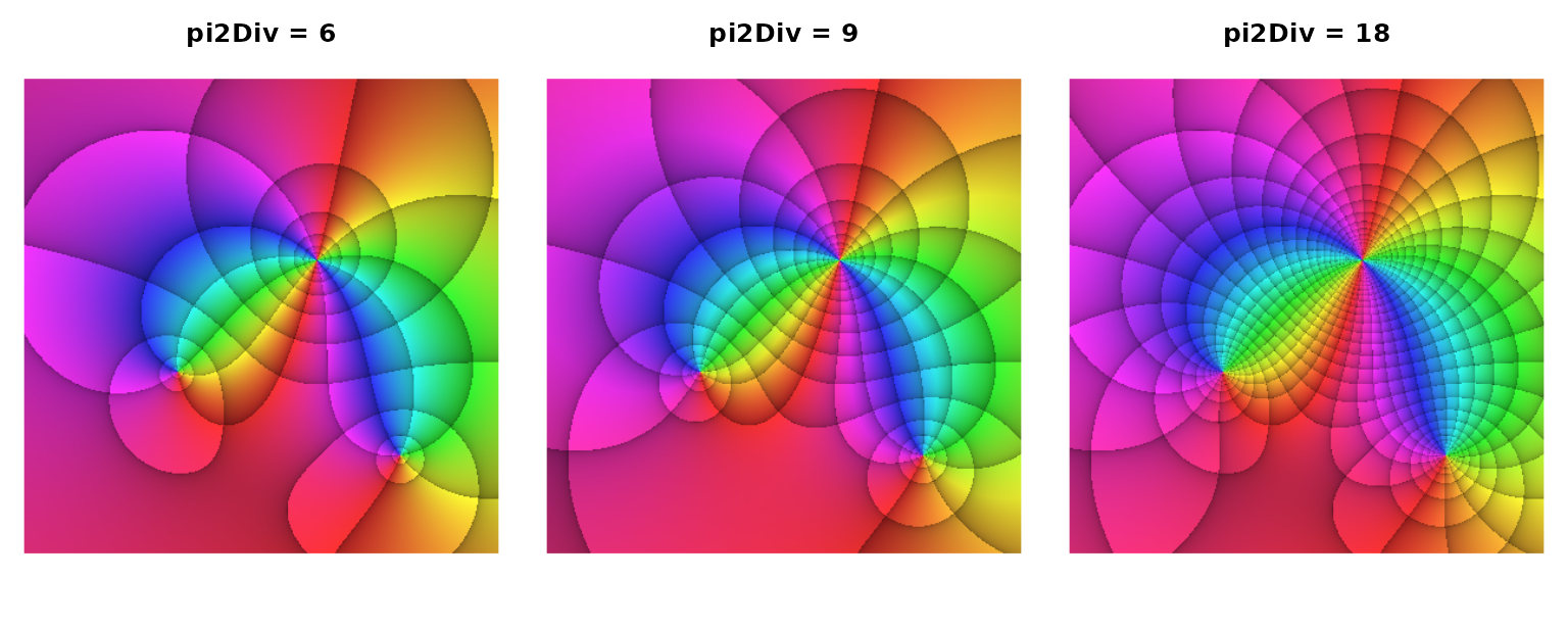

The function \(f(z)=\frac{(3+2\mathrm{i}+z)(-5+5\mathrm{i}+z)}{(-2-2\mathrm{i}+z)^2}\) portrayed with three different settings of pi2Div and pType = "pma".

Evidently, the choice of pi2Div has influenced the density of the iso-modulus lines. This is because, by default, the parameter logBase, which controls how dense the iso-modulus lines are arranged, is linked to pi2Div. As stated above, pi2Div is usually a natural number \(n\:(n \in\mathbb{N})\), and logBase is the real number \(b\:(b\in\mathbb{R})\) which defines the moduli \(r=b^k\:(k\in\mathbb{Z})\) where the reference lines are drawn. When \(n\) is given, the default definition of \(b\) is \(b=\mathrm{e}^{2\pi/n}\). In the default case, \(n=9\), this results in \(b\approx2.009994\). Thus, by default, moving from one iso-modulus line to the adjacent one means almost exactly doubling or halving the modulus, depending on the direction. For the other two cases \(n=6\) and \(n=18\), the resulting values for \(b\) are \(b\approx2.85\) and \(b\approx1.42\), the latter obviously being the square root of \(\mathrm{e}^{2\pi/9}\). For \(n=9\), the modulus (approximately) doubles or halves when traversing two adjacent iso-modulus lines.

Before we demonstrate the special property of this linkage between \(n\) and \(b\), i.e. between pi2Div and logBase, we shortly show, that they can be decoupled in phasePortrait without any complication. In the following example, we want to define the density of the iso-modulus lines in a way that the modulus triples when traversing three zones in the direction of ascending moduli. Clearly, this requires to define logBase as \(b=\sqrt[3]{3}\approx1.44\). Thus, when moving from one iso-modulus line to the next higher one, the modulus has increased by a factor of about \(1.4\). One line further, it has about doubled (\({\sqrt[3]{3}}^{2}\approx2.08\)), and another line further it has exactly tripled. While varying pi2Div exactly as in the previous example, we now keep logBase constant at \(\sqrt[3]{3}\). Run the code below for visualizing this (active 7” x 2.8” screen graphics device suggested, e.g. x11(width = 7, height = 2.8)).

# divide graphics device into three regions and adjust plot margins 
op <- par(mfrow = c(1, 3), mar = c(0.2, 0.2, 0.4, 0.2))
for(n in c(6, 9, 18)) {
  phasePortrait("(3+2i+z)*(-5+5i+z)/(-2-2i+z)^2", xlim = c(-8.5, 8.5), ylim = c(-8.5, 8.5),
                pi2Div = n, logBase = sqrt(3), pType = "pma", axes = FALSE)
  # separate title call (R base graphics) for nicer line adjustment, just cosmetics
  title(paste("pi2Div = ", n, ", logBase = 3^(1/3)", sep = ""), line = -1.2) 
}
par(op) # reset graphics parameters to previous values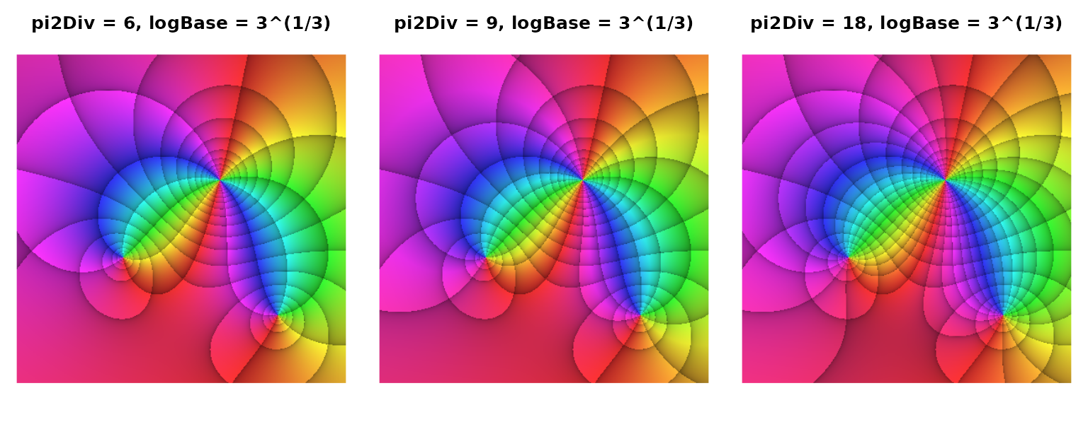

The function \(f(z)=\frac{(3+2\mathrm{i}+z)(-5+5\mathrm{i}+z)}{(-2-2\mathrm{i}+z)^2}\) portrayed with decoupled settings of pi2Div and logBase.

In order to understand why by default the parameters pi2Div and logBase are linked as described above, we consider the exponential function \(f(z)=\mathrm{e}^z\). We can write \(z=r\cdot(\cos\varphi+\mathrm{i}\cdot\sin\varphi)\) and thus \(f(z)=\mathrm{e}^{r\cdot(\cos\varphi+\mathrm{i}\cdot\sin\varphi)}\) or \(w=f(z)=\mathrm{e}^{r\cdot\cos\varphi}\cdot\mathrm{e}^{\mathrm{i}\cdot r\cdot\sin\varphi}\). The modulus of \(w\) is \(\mathrm{e}^{r\cdot\cos\varphi}\) and its argument is \(r\cdot\sin\varphi\) with \(\Re(z)=r\cdot\cos\varphi\) and \(\Im(z)=r\cdot \sin\varphi\). So, the modulus and the argument of \(w=\mathrm{e}^z\) depend solely on the real and the imaginary part of \(z\), respectively. This can be easily verified with a phase portrait of \(f(z)=\mathrm{e}^z\). Run the code below for displaying the phase portrait (active 7” x 7” screen graphics device suggested, e.g. x11()). Note that in the call to phasePortrait we hand over the exp function directly as an object. Alternatively, the quoted strings "exp(z)" or "exp" can be used as well (see section ways to provide functions to phasePortrait below).

op <- par(mar = c(5.1, 4.1, 2.1, 2.1), cex = 0.8) # adjust plot margins 
                                                  # and general text size
phasePortrait(exp, xlim = c(-8.5, 8.5), ylim = c(-8.5, 8.5), pType = "pm",
              xlab = "real", ylab = "imaginary")
par(op) # reset graphics parameters to previous values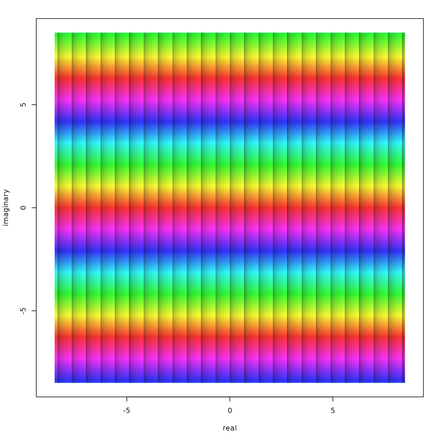                         

Phase portrait of the function \(f(z)=\mathrm{e}^z\) in the window \(\left|\Re(z)\right| < 8.5\) and \(\left|\Im(z)\right| < 8.5\) with iso-modulus lines.

If we now define the argument pi2Div as a number \(n\:(n\in\mathbb{N})\) and use it for determining the angular difference \(\Delta\varphi=\frac{2\pi}{n}\) between two subsequent phase angle reference lines, our default link between pi2Div and logBase (which is the ratio \(b\) of the moduli at two subsequent iso-modulus lines) establishes \(b=\mathrm{e}^{\Delta\varphi}\). This means, if we add \(\Delta\varphi\) to the argument of any \(w=\mathrm{e}^z\:(z\in\mathbb{C})\) or increase its modulus by the factor \(\mathrm{e}^{\Delta\varphi}\), both are equidistant reference line steps in a plot of \(f(z)=\mathrm{e}^z\). We visualize this with the following R code:

# divide graphics device into three regions and adjust plot margins 
op <- par(mfrow = c(1, 3), mar = c(0.2, 0.2, 0.4, 0.2))
for(n in c(6, 9, 18)) {
  phasePortrait("exp(z)", xlim = c(-8.5, 8.5), ylim = c(-8.5, 8.5),
                pi2Div = n, pType = "pma", axes = FALSE)
  # separate title call (R base graphics) for nicer line adjustment, just cosmetics
  title(paste("pi2Div = ", n, ", logBase = exp(2*pi/pi2Div)", sep = ""), 
        line = -1.2, cex.main = 0.9) 
}
par(op) # reset graphics parameters to previous values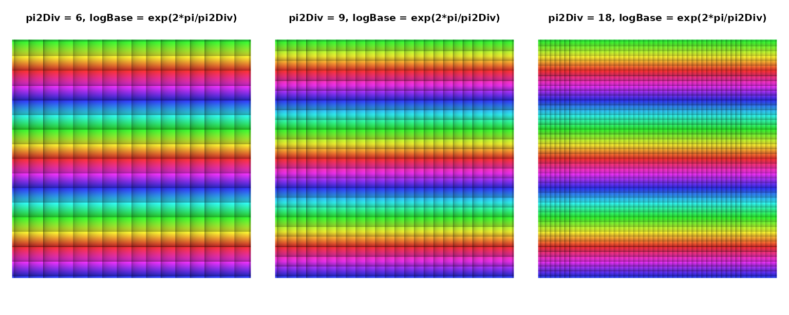

The function \(f(z)=\mathrm{e}^z\) portrayed with the default coupling of pi2Div and logBase as implemented in phasePortrait.

As expected, the default coupling of both arguments produces square patterns when applied to a phase portrait of the exponential function which can, insofar, serve as a visual reference. Recall, that equidistant modulus reference lines (in ascending order) indicate an exponentially growing modulus. In the middle phase portrait one such steps means (approximately) doubling the modulus. From the left to the right, the plot covers 24 of these steps, indicating a total increase of the modulus by factor \(2^{24}\) which amounts to almost 17 millions.

Fine tuning shading and contrast

For optimizing visualization in a technical sense, as well as for aesthetic purposes, it may be useful to adjust shading and contrast of the argument and modulus reference zones mentioned above. This is done by modifying the parameters darkestShade (\(s\)) and lambda (\(\lambda\)) when calling phasePortrait. These two parameters can be used to steer the transition from the lower to the uper edge of a reference zone. They address the v-value of the hsv color model, which can take values between 0 and 1, indicating maximum darkness (black), and no shading at all, respectively. Hereby, \(s\) gives the v-value at the lower edge of a reference zone, and \(\lambda\) determines the interpolation from there to the upper edge, where no shading is applied. The intended use is \(\lambda > 0\) where small values sharpen the contrast between shaded and non-shaded zones and vice versa. Exactly, the shading value \(v\) is calculated as: \[ v = s + (1-s)\cdot x^{1/\lambda} \] For modulus zone shading at a point \(z\) in the complex plane when portraying a function \(f(z)\), \(x\) is the fractional part of \(\log_b{f(z)}\), with the base \(b\) being the parameter logBase that defines the modulus reference zoning (see above). For shading argument reference zones, \(x\) is simply the difference between the upper and the lower angle of an argument reference zone, linearly mapped to the range \([0, 1[\). The following code generates a \(3\times3\) matrix of phase portraits of \(f(z)=\tan{z^2}\) with \(\lambda\) and \(s\) changing along the rows and columns, respectively. Run the code for visualizing these concepts (active 7” x 7” screen graphics device suggested, e.g. x11()).

op <- par(mfrow = c(3, 3), mar = c(0.2, 0.2, 0.2, 0.2))
for(lb in c(0.1, 1, 10)) {
  for(dS in c(0, 0.2, 0.4)) {
    phasePortrait("tan(z^2)", xlim = c(-1.7, 1.7), ylim = c(-1.7, 1.7), 
                  pType = "pm", darkestShade = dS, lambda = lb, 
                  axes = FALSE, xaxs = "i", yaxs = "i")
  }
}
par(op)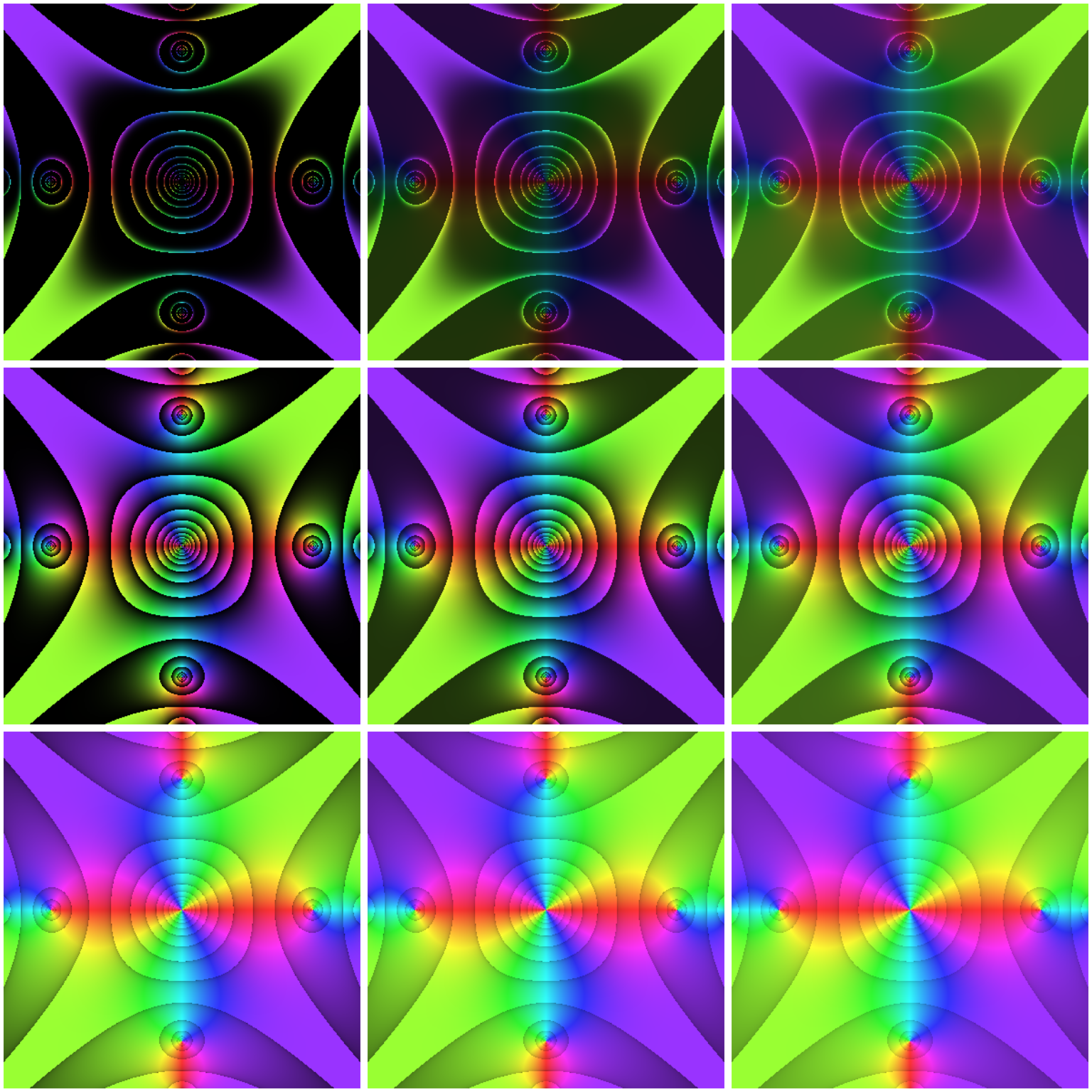

Tuning reference zone contrast with the parameters darkestShade (column-wise, 0, 0.2, 0.4), and lambda (row-wise, 0.1, 1, 10).

Additional possibilities exist for tuning the interplay of modulus and argument reference zones when they are used in combination; this can be controlled with the parameter gamma when calling phasePortrait). The maximum brightness of the colours in a phase portrait is adjustable with the parameter stdSaturation (see documentation of phasePortrait; we will also get back to these points in the chapter aesthetic hints below).

Be aware of branch cuts

When exploring functions with phasePortrait, discontinuities of certain functions can become visible as abrupt color changes. Typical examples are integer root functions which, for a given point \(z, z\in\mathbb{C}\setminus\lbrace0\rbrace\) in the complex plane, can attain \(n\) values with \(n\) being the root’s degree. It takes, so to speak, \(n\) full cycles around the origin of the complex plane in order to cover all values obtained from a function \(f(z)=z^{1/n}, n\in\mathbb{N}\). This is illustrated for the third root function in the figure below.

op <- par(mfrow = c(1, 3), mar = c(0.4, 0.2, 0.2, 0.2))
for(k in 0:2) {
  FUNstring <- paste0("z^(1/3) * exp(1i * 2*pi/3 * ", k, ")")
  phasePortrait(FUN = FUNstring, 
                xlim = c(-1.5, 1.5), ylim = c(-1.5, 1.5), pi2Div = 12, 
                axes = FALSE)
  title(sub = paste0("k = ", k), line = -1)
  # emphasize branch cut with a dashed line segment
  segments(-1.5, 0, 0, 0, lwd = 2, lty = "dashed") 
  # draw colored arrows
  upperCol <- switch(as.character(k),
                     "0" = "black", "1" = "red", "2" = "green")
  lowerCol <- switch(as.character(k),
                     "0" = "green", "1" = "black", "2" = "red")
  arrows(x0 = c(-1.2), y0 = c(1, -1), y1 = c(0.2, -0.2), 
         lwd = 2, length = 0.1, col = c(upperCol, lowerCol))
}
par(op)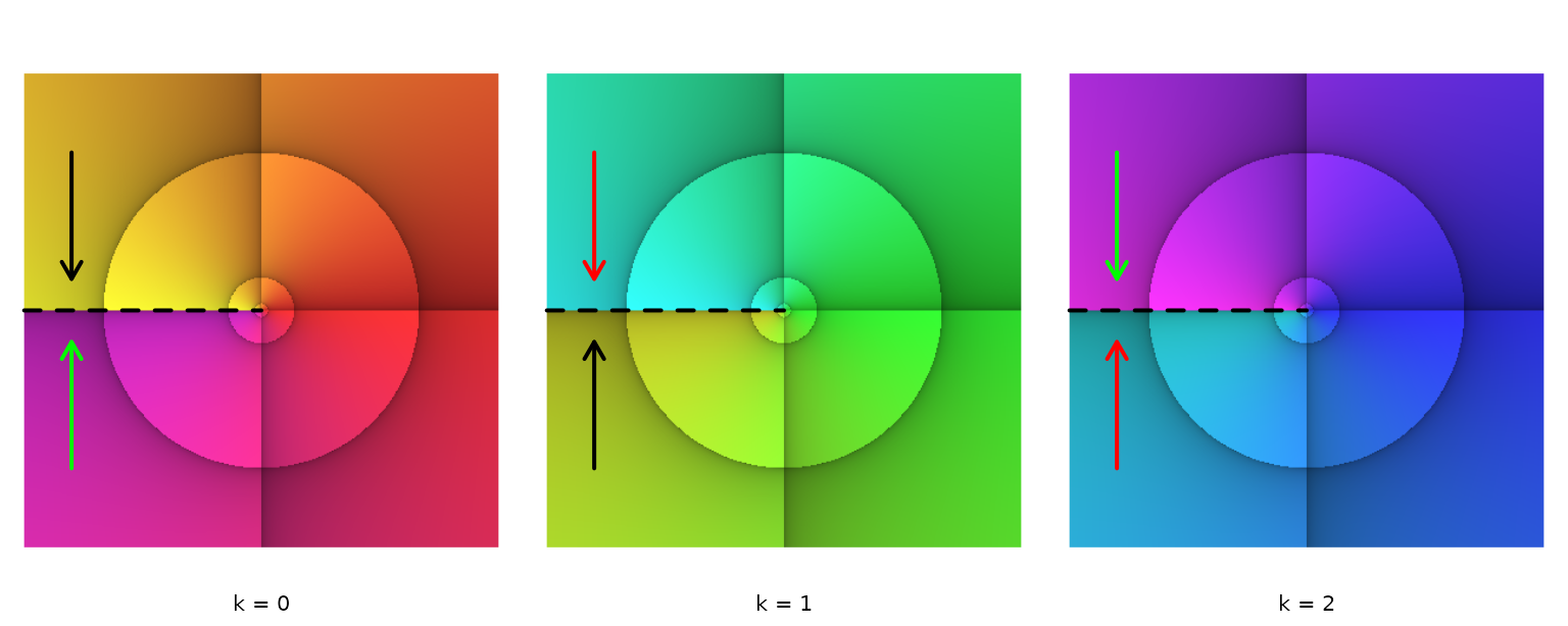

Three phase portraits with branch cuts (dashed line), illustrating the three values of \(f(z)=z^{1/3}\), \(z \in \mathbb{C} \setminus \lbrace 0 \rbrace\). The transitions between the phase portraits are indicated by same-coloured arrows pointing at the branch cuts.

First, have a look at the leftmost diagram. Note that the argument reference lines have been adjusted to represent angle distances of \(30°\), i.e. pi2Div = 12. Most noticeable is the abrupt color change from yellow to magenta along the negative real axis (emphasized with a dashed line). This is what is called a branch cut, and it suggests that our picture of the function \(f(z)=z^{1/3}\) is not complete. As the three third roots of any complex number \(z=r\cdot\mathrm{e}^{\mathrm{i}\varphi}, z\in\mathbb{C}\setminus\lbrace0\rbrace\) are \(r^{1/3}\cdot\mathrm{e}^{\mathrm{i}\cdot(\varphi+k\cdot2\pi)/3}; k=0,1,2; \varphi\in\left[0,2\pi\right[\), we require three different phase portraits, one for each \(k\), as shown in the figure above. With the argument reference line distance being \(30°\), it is easy to see that each phase portrait covers a total argument range of \(120°\), i.e. \(2\pi/3\).

Obviously, each of the three portraits has a branch cut along the negative real axis, and the colors at the branch cuts show, where the transitions between the phase portraits have to happen. In the figure, we have illustrated this by arrows pointing to the branch cuts. Same-colored arrows in different phase portraits indicate the transitions. Thus, the first phase portrait (\(k = 0\)) links to the second (\(k = 1\)) in their yellow zones (black arrows); the second links to the third (\(k = 2\)) in their blue zones (red arrows), and the third links back to the first in their magenta zones (green arrows). Actually, one could imagine to stack the three face portraits in ascending order, cut them at the dashed line, and glue the branch cuts together according to the correct transitions. The resulting object is a Riemann surface with each phase portrait being a ‘sheet.’ See more about this fascinating concept in Wegert (2012), Chapter7.

While the function \(f(z)=z^{1/3}\) could be fully covered with three phase portraits, \(f(z)=\log z\) has an infinite number of branches. As the (natural) logarithm of any complex number \(z=r\cdot\mathrm{e}^{i\cdot\varphi}, r>0\) is \(\log z=\log r+\mathrm{i}\cdot\varphi\), it is evident that the imaginary part of \(\log z\) increases linearly with the argument of \(z\), \(\varphi\). In terms of phase portraits, this means an infinite number of stacked ‘sheets’ in either direction, clockwise and counterclockwise. Neighboring sheets connect at a branch cut. We illustrate this below with a phase portrait of \(\log z=\log r+\mathrm{i}\cdot(\varphi+k\cdot2\pi), r > 0, \varphi\in\left[0,2\pi\right[\) for \(k=-1, 0, 1\).

op <- par(mfrow = c(1, 3), mar = c(0.4, 0.2, 0.2, 0.2))
for(k in -1:1) {
  FUNstring <- paste0("log(Mod(z)) + 1i * (Arg(z) + 2 * pi * ", k, ")") 
  phasePortrait(FUN = FUNstring, pi2Div = 36,
                xlim = c(-2, 2), ylim = c(-2, 2), axes = FALSE)
  segments(-2, 0, 0, 0, col = "white", lwd = 1, lty = "dashed")
  title(sub = paste0("k = ", k), line = -1)
}  
par(op)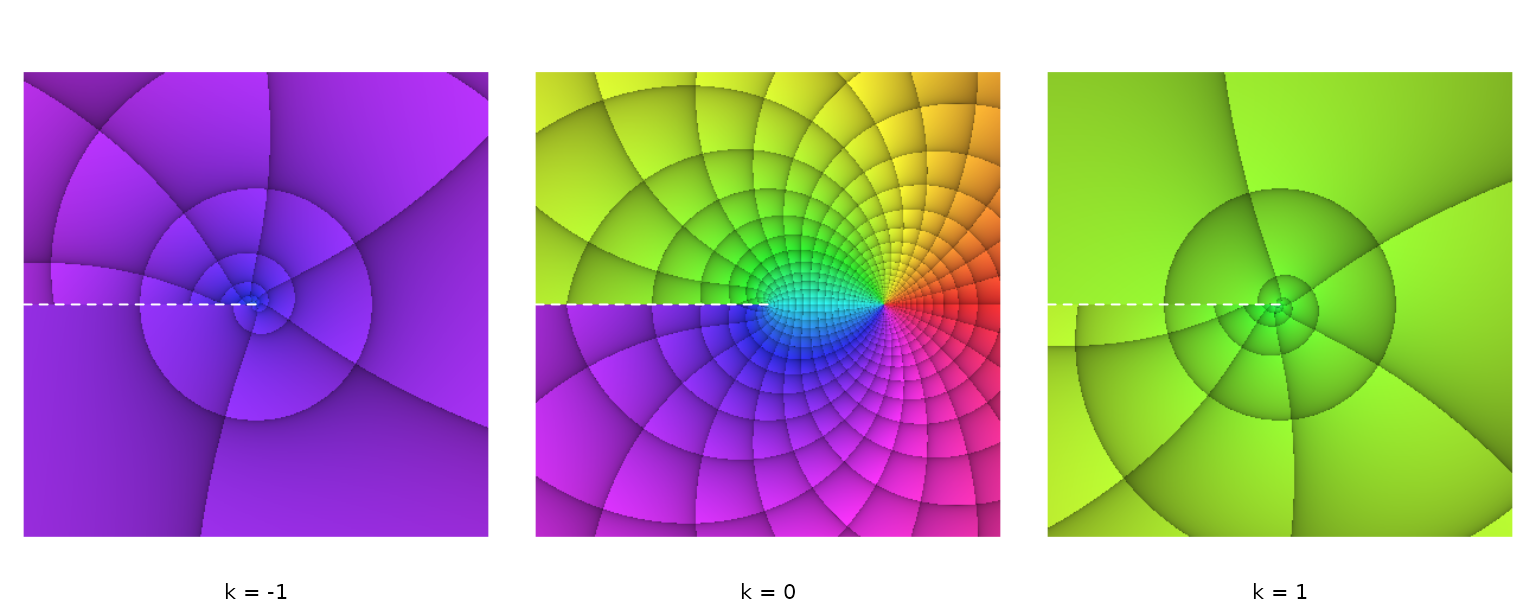

Three branches of \(\log z=\log r+\mathrm{i}\cdot(\varphi + k\cdot2\pi), r>0, \varphi\in\left[0,2\pi\right[\), with \(k=-1,0,1\). The branch cuts are marked with dashed white lines.

Riemann sphere plots

A convenient way to visualize the whole complex number plane is based on a stereographic projection suggested by Bernhard Riemann (see Wegert (2012), p. 20 ff. and p. 39 ff.). The Riemann Sphere is a sphere with radius 1, centered around the origin of the complex plane. It is cut into an upper (northern) and lower (southern) half by the complex plane. By connecting any point on the complex plane to the north pole with a straight line, the line’s intersection with the sphere’s surface marks the location on the sphere where the point is projected onto. Thus, all points inside the unit disk on the complex plane are projected onto the southern hemisphere, the origin being represented by the south pole. In contrast, all points outside the unit disk are projected onto the northern hemisphere, the north pole representing the point at infinity. For visualizing both hemispheres as 2D phase portraits, they have to be projected onto a flat surface in turn.

If we perform a stereographic projection of the southern hemisphere from the north pole to the complex plane (and look at the plane’s upper - the northern - side), this obviously results in a phase portrait on the untransformed complex plane as were all examples shown so far in this text. We can perform an analogue procedure for the northern hemisphere, projecting it from the south pole to the complex plane. We now want to think of the northern hemisphere projection as layered on top of the southern hemisphere projection, for the northern hemisphere, which it depicts, is naturally also on top of the southern hemisphere. If, in a ‘normal’ visualization of the complex plane (orthogonal real and imaginary axes), a point at any location represents a complex number \(z\), a point at the same location in the northern hemisphere projection is mapped into \(1/z\). The origin is mapped into the point at infinity. Technically, this mapping can be easily achieved when calling the function phasePortrait by setting the flag invertFlip = TRUE (default is FALSE). The resulting map is, in addition, rotated counter-clockwise around the point at infinity by an angle of \(\pi\). As Wegert (2012) argues, this way of mapping has a convenient visual effect: Consider two phase portraits of the same function, one made with invertFlip = FALSE and the other one with invertFlip = TRUE. Both are shown side by side (see the pairs of phase portraits in the next two figures below). This can be imagined as a view into a Riemann sphere that has been cut open along the equator and swung open along a hinge in the line \(\Re(z)=1\) (if the southern hemisphere is at the left side) or \(\Re(z)=-1\) (if the northern hemisphere is at the left side). In order to highlight the Riemann sphere in phase portraits if desired, we provide the function riemannMask. Let’s first demonstrate this for the function \(f(z)=z\).

op <- par(mfrow = c(1, 2), mar = rep(0.1, 4))
# Southern hemisphere
phasePortrait("z", xlim = c(-1.4, 1.4), ylim = c(-1.4, 1.4), 
              pi2Div = 12, axes = FALSE)
riemannMask(annotSouth = TRUE)
# Northern hemisphere
phasePortrait("z", xlim = c(-1.4, 1.4), ylim = c(-1.4, 1.4), 
              pi2Div = 12, axes = FALSE, invertFlip = TRUE)
riemannMask(annotNorth = TRUE)
par(op)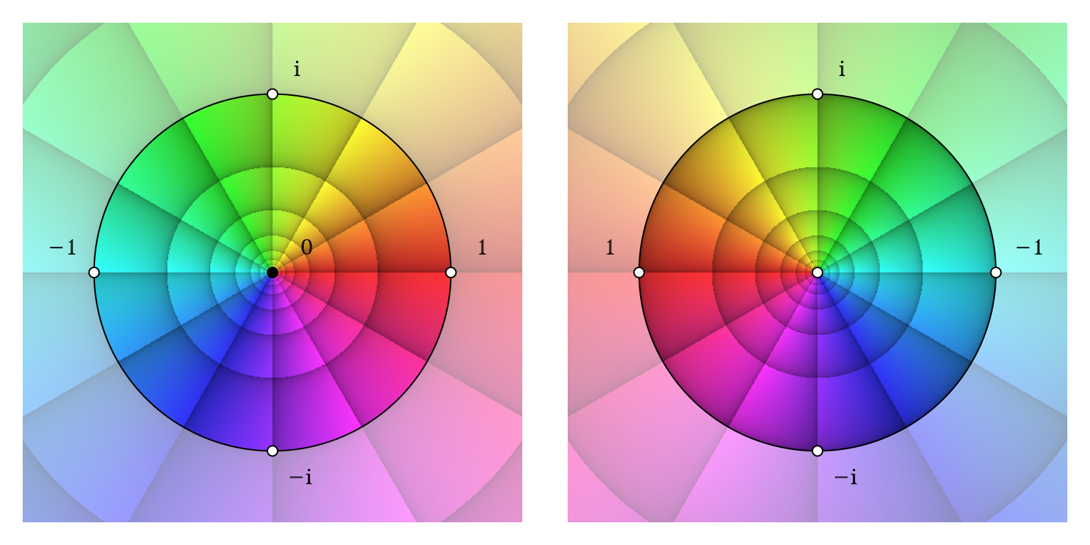

Mapping the complex number plane on the Riemann sphere. Left: lower (southern) hemisphere; right upper (northern hemisphere). Folding both figures face to face along a vertical line in the middle between them can be imagined as closing the Riemann sphere.

The function riemannMask provides several options, among others adjusting the mask’s transparency or adding annotations to landmark points (see the function’s documentation). In the next example, we will use it without any such features. Consider the following function: \[ f(z)=\frac{(z^{2}+\frac{1}{\sqrt{2}}+\frac{\mathrm{i}}{\sqrt{2}})\cdot(z+\frac{1}{2}+\frac{\mathrm{i}}{2})}{z-1} \] This function has two zeroes exactly located on the unit circle, \(z_1=\mathrm{e}^{\mathrm{i}\frac{5\pi}{8}}\), and \(z_2=\mathrm{e}^{\mathrm{i}\frac{13\pi}{8}}\). Moreover, it has another zero inside the unit circle, \(z_3=\frac{1}{\sqrt{2}}\cdot\mathrm{e}^{\mathrm{i}\frac{5\pi}{4}}\). Equally obvious, it has a pole exactly on the unit circle, \(z_4=1\). Less obvious, it has a double pole, \(z_5\), at the point at infinity. The code required for producing the following figure looks somewhat bulky, but most lines are required for annotating the zeroes and poles. Note that the real axis coordinates of the northern hemisphere’s annotation do not have to be multiplied with \(-1\) in order to take into account the rotation of the inverted complex plane. By calling phasePortrait with invertFlip = TRUE the coordinate system of the plot is already set up correctly and will remain so for subsequent operations.

op <- par(mfrow = c(1, 2), mar = c(0.1, 0.1, 1.4, 0.1))
# Define function
FUNstring <- "(z^2 + 1/sqrt(2) * (1 + 1i)) * (z + 1/2*(1 + 1i)) / (z - 1)"
# Southern hemisphere
phasePortrait(FUNstring, xlim = c(-1.2, 1.2), ylim = c(-1.2, 1.2), 
              pi2Div = 12, axes = FALSE)
riemannMask()
title("Southern Hemisphere", line = 0)
# - annotate zeroes and poles
text(c(cos(5/8*pi), cos(13/8*pi), cos(5/4*pi)/sqrt(2), 1),
     c(sin(5/8*pi), sin(13/8*pi), sin(5/4*pi)/sqrt(2), 0), 
     c(expression(z[1]), expression(z[2]), expression(z[3]), expression(z[4])), 
     pos = c(1, 2, 4, 2), offset = 1, col = "white")
# Northern hemisphere
phasePortrait(FUNstring, xlim = c(-1.2, 1.2), ylim = c(-1.2, 1.2), 
              pi2Div = 12, axes = FALSE, invertFlip = TRUE)
riemannMask()
title("Northern Hemisphere", line = 0)
# - annotate zeroes and poles
text(c(cos(5/8*pi), cos(13/8*pi), cos(5/4*pi)*sqrt(2), 1, 0),
     c(sin(5/8*pi), sin(13/8*pi), sin(5/4*pi)*sqrt(2), 0, 0), 
     c(expression(z[1]), expression(z[2]), expression(z[3]), 
       expression(z[4]), expression(z[5])), 
     pos = c(1, 4, 3, 4, 4), offset = 1, 
     col = c("white", "white", "black", "white", "white"))
par(op)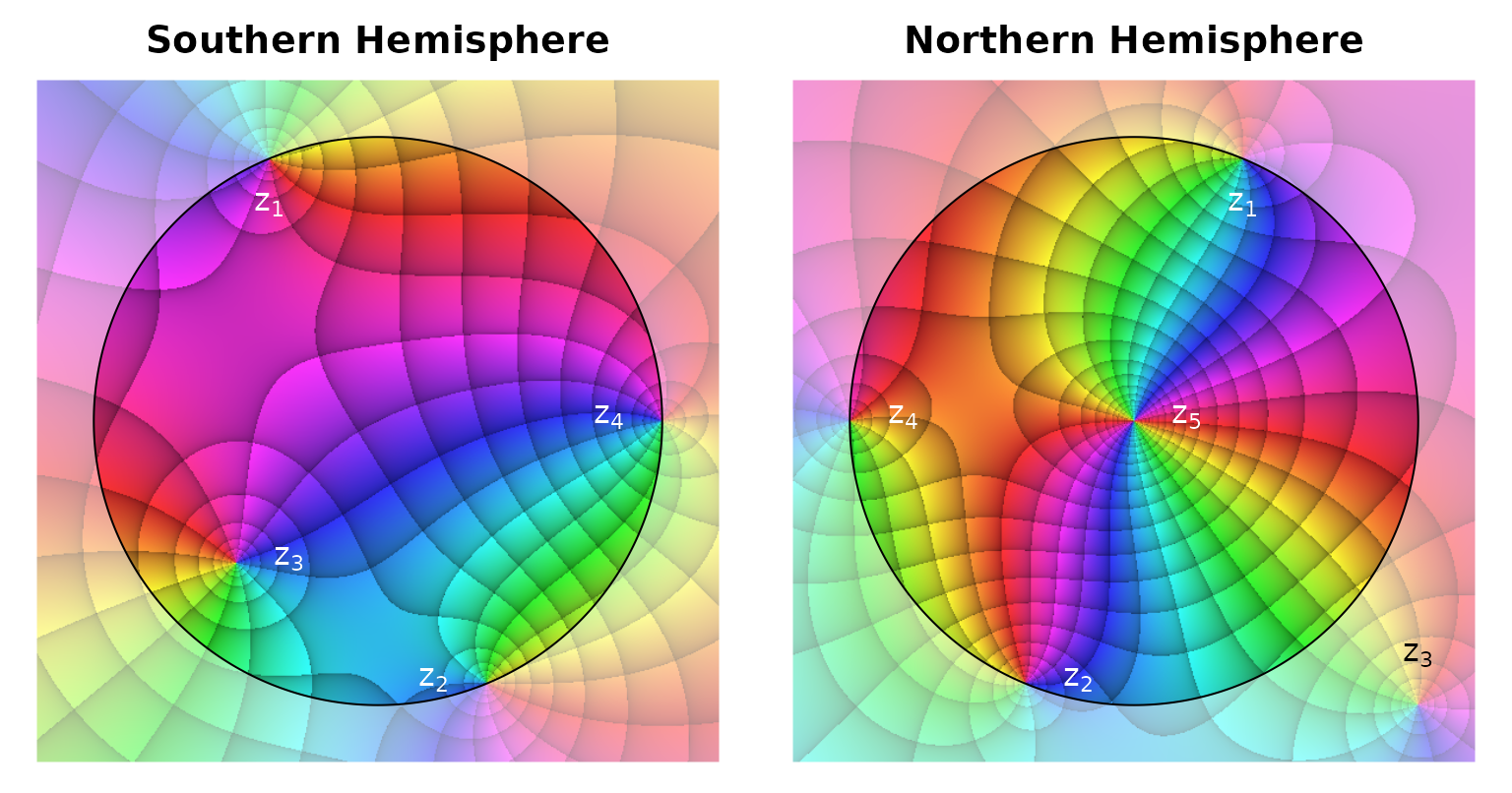

Riemann sphere plot of the function \(f(z)=\frac{(z^{2}+\frac{1}{\sqrt{2}}+\frac{\mathrm{i}}{\sqrt{2}})\cdot(z+\frac{1}{2}+\frac{\mathrm{i}}{2})}{z-1}\). Annotated are the zeroes \(z_1\), \(z_2\), \(z_3\), and the poles \(z_4\), \(z_5\).

With some consideration it becomes quite easy to see that both phase portraits are kind of everted versions of each other. What is inside the unit disk in the left phase portrait is outside in the right one, and vice versa. If you mentally visualize both unit disks touching in, e.g., point \(z_4\) and one disk rolling along the edge of the other, you will see immediately how one disk continues the picture shown in the other. Having the ‘Riemann Mask’ somewhat transparent is helpful for orientation (see the function’s documentation). Note, how the zeroes \(z_{1, 2}\) and the pole \(z_4\) which are located exactly on the unit circle continue outside the unit disk on ‘their own’ plane and in the other unit disk. Note also, that on both hemispheres zeroes and poles can be identified by the same sequence of colors: When circling counter-clockwise around the point of interest, a zero will always exhibit the color sequence red, yellow, green, blue, magenta, red …, while this order will always be reverted for a pole. As the pole at the point at infinity (\(z_5\)) is a double pole, the color sequence is run through twice during one turn around the pole. As the zero \(z_3\) is inside the unit disk representing the southern hemisphere, it lies outside the northern hemisphere disk, but it is still visible on the continuation of the inverted (and rotated) complex plane (belonging to the northern hemisphere) outside the unit disk. Observe, how the grid lines in the vicinity of \(z_3\) merge when passing from one unit disk to the other.

Fractals

While visualizing fractals is not among the original purposes of this package, phasePortrait allows for an unusual way of displaying such that are functions of complex numbers. Classic examples are the Mandelbrot set and the Julia set, and this package provides the functions mandelbrot and juliaNormal (implemented in C++) for supporting visualization. The mandelbrot set comprises all complex numbers \(z\) for which the sequence \(a_{n+1}=a_n^{2}+z\) with \(a_0=0\) remains bounded for all \(n\in\mathbb{N_0}\). Normal julia sets are closely related to the Mandelbrot set. They comprise all complex numbers \(z\) for which the sequence \(a_{n+1}=a_n^2+c\) with \(a_0=z\) remains bounded for all \(n\in\mathbb{N_0}\). The parameter \(c\) is a complex number, and interesting visualizations with this package (i.e. other than a blank screen) are only obtained for \(c\) being an element of the Mandelbrot set. For the author’s taste, the Julia set visualizations look best and are most interesting when \(c\) is located near the border of the Mandelbrot set. The classic visualizations of the Mandelbrot and the Julia set use a uniform color (usually black) for all points which belong to the set and color the points outside the set dependent on how quickly they diverge. Visualizations with phasePortrait, in contrast, color the points inside the sets by the argument and modulus of the number to which the series described above converges (or, more precisely, at which the iteration terminates). While the results are visually appealing (please try the code examples we provide below), they are not unambiguous, as the sequences that define the sets do not always converge to one single value, but to limit cycles.

The following code plots an overview picture of the Mandelbrot set. Note that the function mandelbrot is called with a considerably low value (30) for the parameter itDepth which defines the number of iterations to be calculated (default is 500). This is because we are using phasePortrait for plotting into a graphics window with a comparatively low resolution (see section defining image quality for how to obtain high-quality phase portraits). While a high number of iterations produces a more accurate representation of the set, the resulting filigree structures might become hardly visible or even invisible when the resolution to be plotted on is low.

op <- par(mar = c(0, 0, 0, 0))        # Do not leave plot margins
phasePortrait(mandelbrot, moreArgs = list(itDepth = 30),
              xlim = c(-2, 1), ylim = c(-1, 1),
              hsvNaN = c(0, 0, 0),    # black color for points outside the set 
              axes = FALSE,           # No coordinate axes   
              xaxs = "i", yaxs = "i") # No space between plot region and plot
par(op)                               # Set graphics parameters to original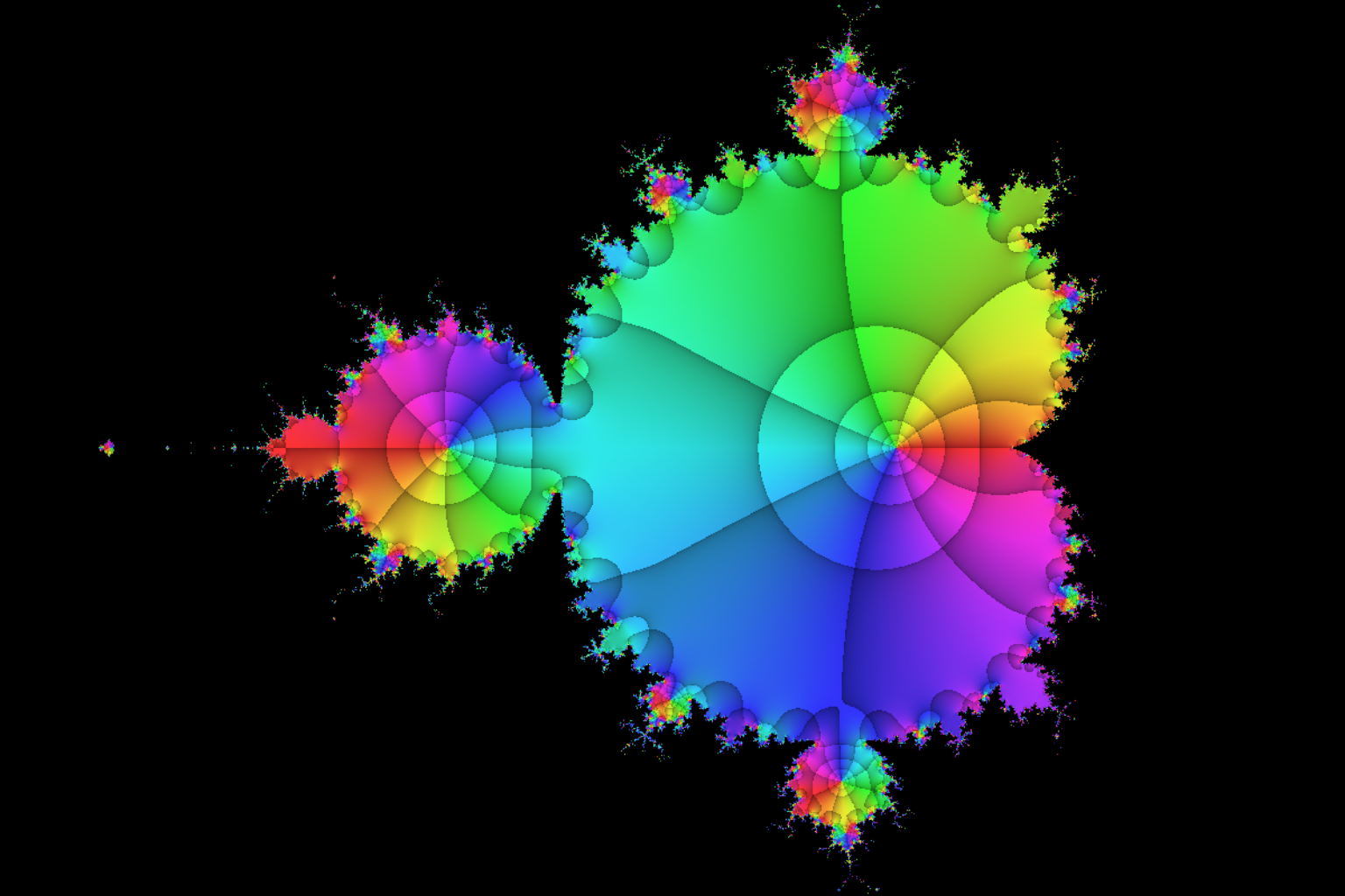

With the code example below we plot a cutout of the Mandelbrot set into a png file with a resolution of 600 dpi using the default number of iterations (500). We are using a few features that are just commented here, but will be explained below in the section aesthetic hints. Other graphics file formats can be used in almost the same way. Type ?png in order to see all formats and how to call them. See also section defining image quality.

res  <- 600 # set resolution to 600 dpi
# open png graphics device with in DIN A4 format
# DIN A format has an edge length ratio of sqrt(2)
png("Mandelbrot Example.png", 
    width = 29.7, height = 29.7/sqrt(2), # DIN A4 landscape
    units = "cm", 
    res = res)                   # resolution is required
op   <- par(mar = c(0, 0, 0, 0)) # set graphics parameters - no plot margins
xlim <- c(-1.254, -1.248)        # horizontal (real) plot limits  
# the function below adjusts the imaginary plot limits to the
#   desired ratio (sqrt(2)) centered around the desired imaginary value
ylim <- ylimFromXlim(xlim, centerY = 0.02, x_to_y = sqrt(2))
phasePortrait(mandelbrot,
              xlim = xlim, ylim = ylim,
              hsvNaN = c(0, 0, 0),    # Black color for NaN results
              xaxs = "i", yaxs = "i", # suppress R's default axis margins
              axes = FALSE,           # do not plot axes
              res = res)              # resolution is required
par(op)   # reset graphics parameters
dev.off() # close graphics device and complete the png file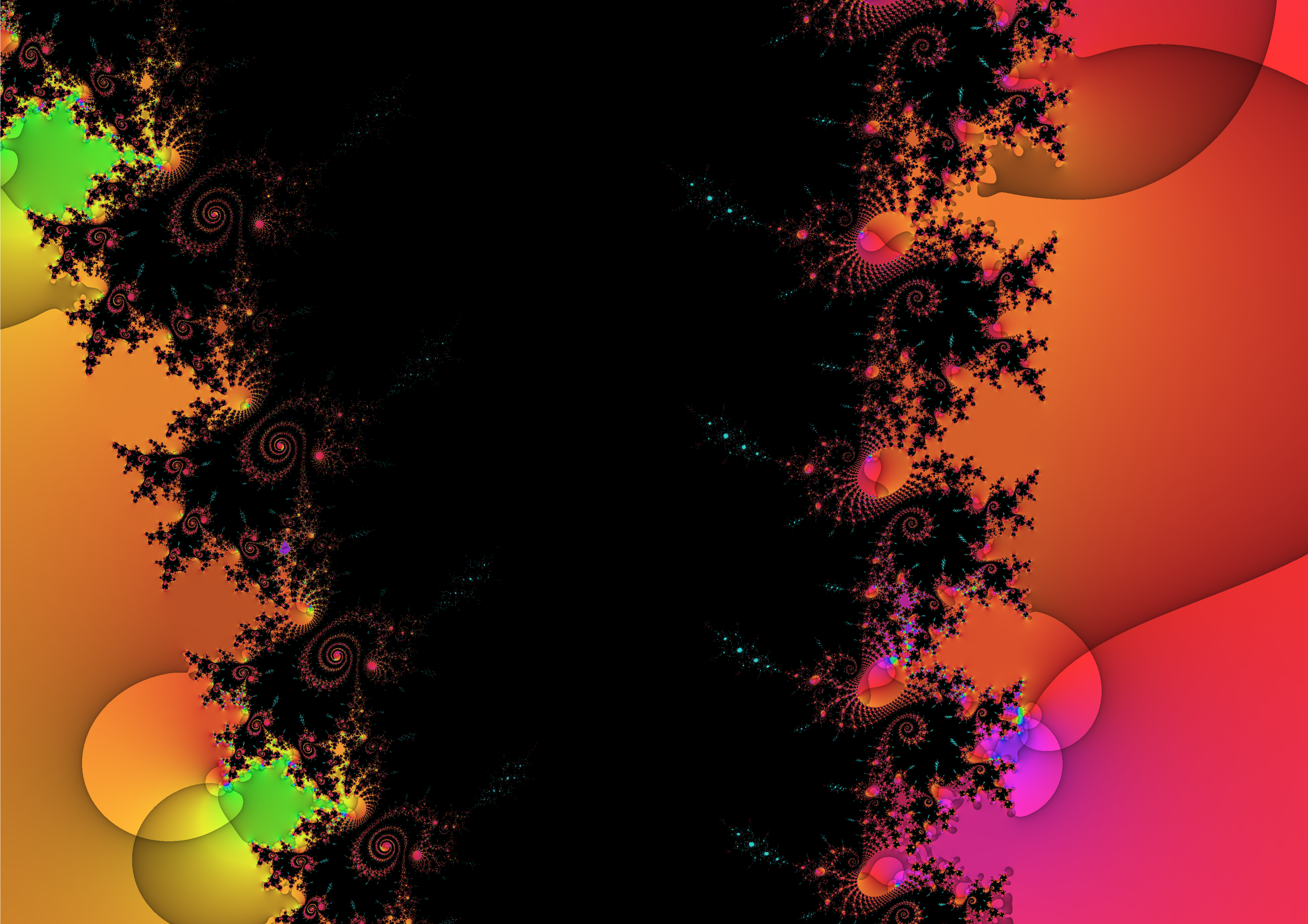

Inside the same technical setting, the following two examples plot Julia sets into a png file.

res <- 600
png("Julia Example 1.png", width = 29.7, height = 29.7/sqrt(2),
    units = "cm", res = res)
op <- par(mar = c(0, 0, 0, 0))
xlim <- c(-1.8, 1.8)
ylim <- ylimFromXlim(xlim, centerY = 0, x_to_y = sqrt(2))
phasePortrait(juliaNormal,
              # see documentation of juliaNormal about the arguments
              #  c and R_esc
              moreArgs = list(c = -0.09 - 0.649i, R_esc = 2),
              xlim = xlim, ylim = ylim,
              hsvNaN = c(0, 0, 0),
              xaxs = "i", yaxs = "i",
              axes = FALSE,
              res = res)
par(op)
dev.off()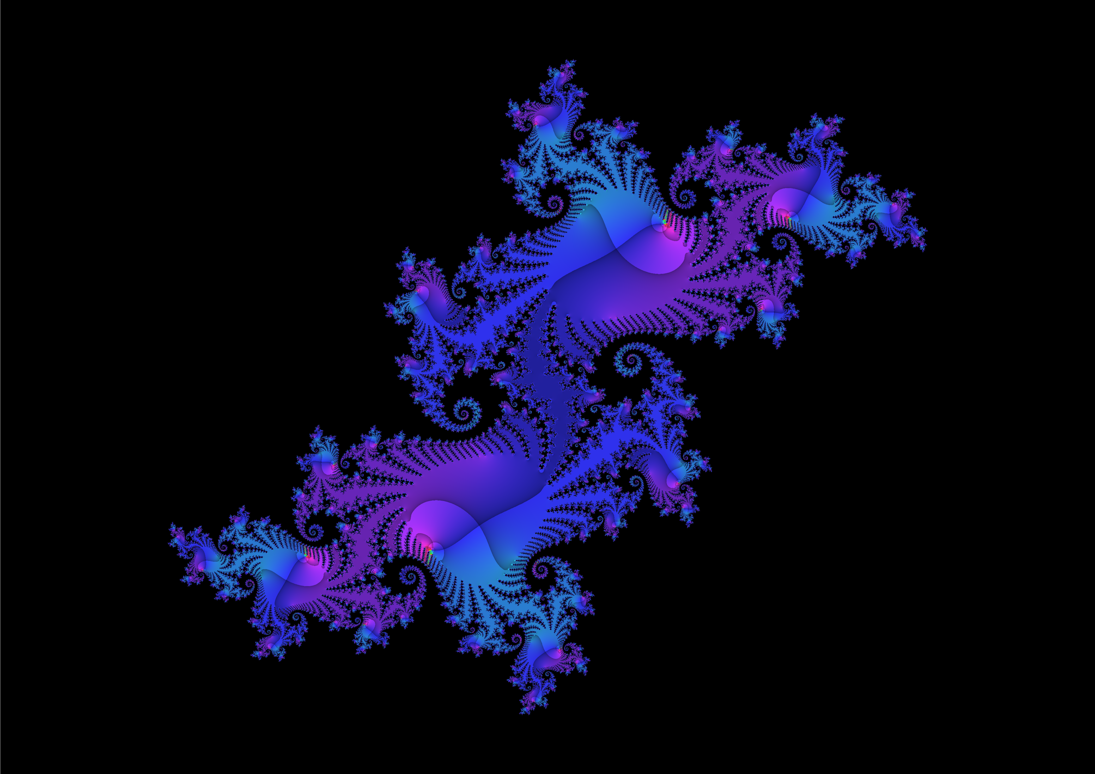

res <- 600
png("Julia Example 2.png", width = 29.7, height = 29.7/sqrt(2),
    units = "cm", res = res)
op <- par(mar = c(0, 0, 0, 0))
xlim <- c(-0.32, 0.02)
ylim <- ylimFromXlim(xlim, center = -0.78, x_to_y = sqrt(2))
phasePortrait(juliaNormal, 
              # see documentation of juliaNormal about the arguments
              #  c and R_esc
              moreArgs = list(c = -0.119 - 0.882i, R_esc = 2),
              xlim = xlim, ylim = ylim,
              hsvNaN = c(0, 0, 0),
              xaxs = "i", yaxs = "i",
              axes = FALSE,
              res = res)
par(op)
dev.off()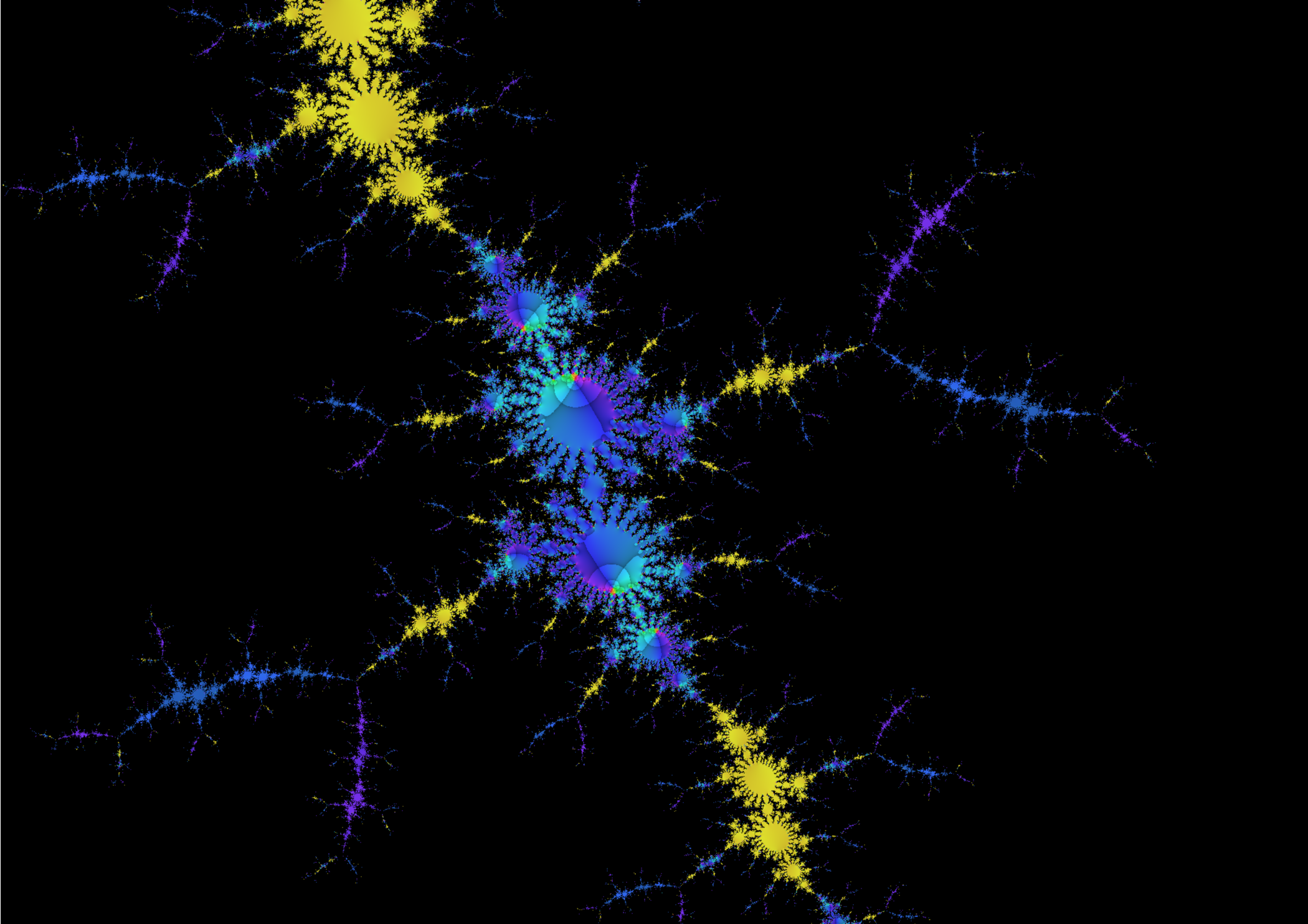

Phase portraits based on a polar chessboard

Since version 1.1.0, viscomplexr provides the function phasePortraitBw which allows for creating two-color phase portraits of complex functions based on a polar chessboard grid (cf. Wegert (2012), p. 35). Compared to the full phase portraits that can be made with phasePortrait, two-color portraits omit information. Especially in combination with full phase portraits they can be, however, very helpful tools for interpretation. Besides, two-color phase portraits have a special aesthetic appeal which is worth exploring for itself. In its parameters and its mode of operation, phasePortraitBw is very similar to phasePortrait (see the documentations of both functions for details). The parameters pi2Div and logBase have exactly the same effect as with phasePortrait. Instead of the parameter pType, phasePortraitBw has the parameter bwType which allows for the three settings “m,” “a,” and “ma.” These produce two-color phase portraits which take into account the modulus only, the argument (phase angle), only, and the combination of both, respectively. Plots made with the latter option show a chessboard-like color alteration over the tiles resulting from the intersection of modulus and argument zones. The following code maps the complex plane to itself, comparing all three options of bwType. It also adds a standard phase portrait for comparison.

# Map the complex plane on itself, show all bwType options

op <- par(mfrow = c(2, 2), mar = c(4.1, 4.1, 1.1, 1.1))
for(bwType in c("ma", "a", "m")) {
  phasePortraitBw("z", xlim = c(-2, 2), ylim = c(-2, 2),
                  bwType = bwType,
                  xlab = "real", ylab = "imaginary")
}
# Add normal phase portrait for comparison
phasePortrait("z", xlim = c(-2, 2), ylim = c(-2, 2),
              xlab = "real", ylab = "imaginary",
              pi2Div = 18)         # Use same angular division as is default
                                   # in phasePortraitBw
par(op)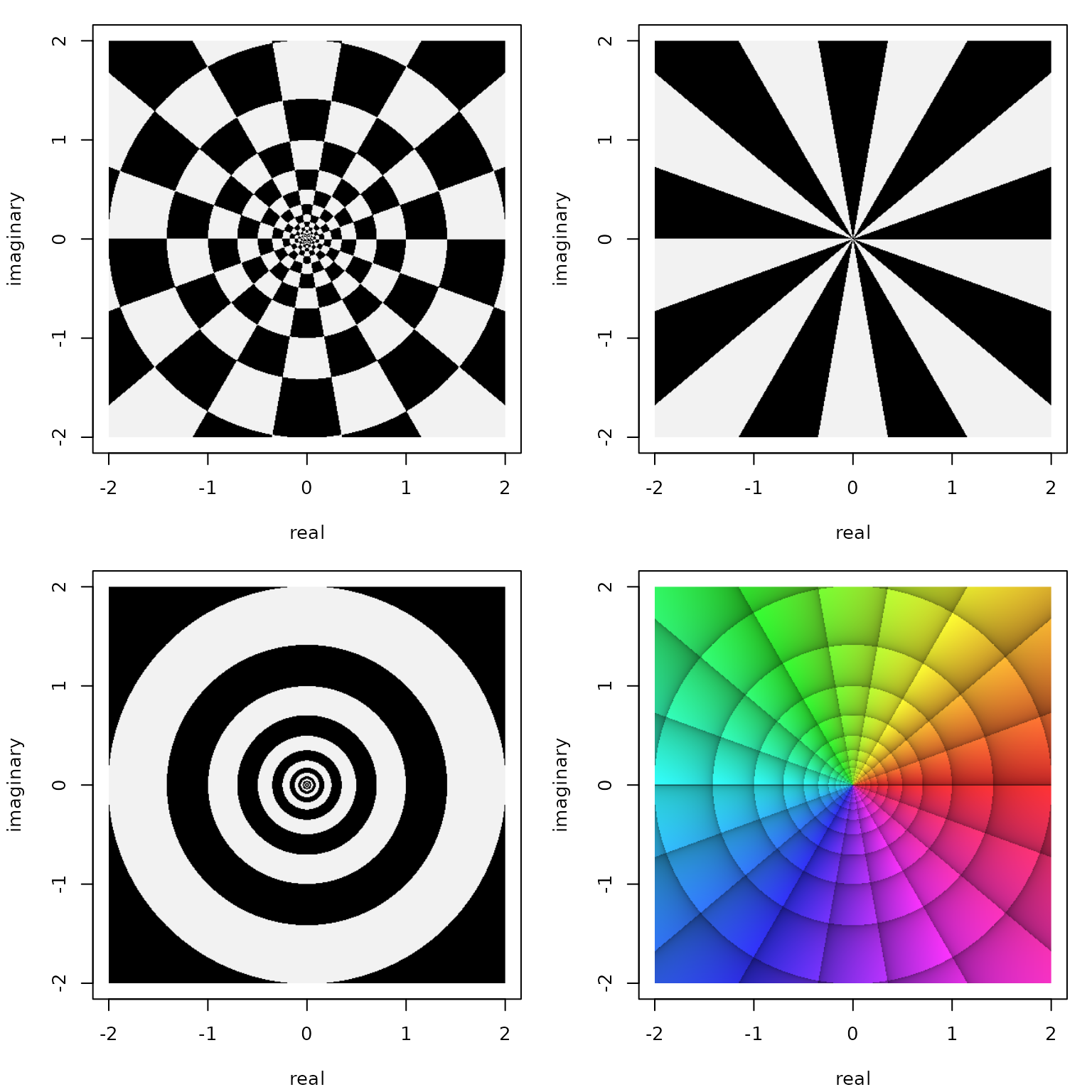

Two color portraits of the function \(f(z)=z\) made with phasePortraitBw and byType ‘ma’ (top left), ‘a’ (top right), and ‘m’ (bottom left) together with a full phasePortrait (bottom right).

Note that the parameter pi2Div should not be chosen as an odd number when working with phasePortraitBw. In this case, the first and the last phase angle zone would obtain the same color, which is probably an undesired effect for most applications. While pi2Div = 9 is the default setting in phasePortrait for good reasons (see above), its default in phasePortraitBw is 18. Also by default, the parameter logBase is linked to pi2Div in the same way as by default in phasePortrait (logBase = exp(2*pi/pi2Div)). So, if defaults for both, phasePortrait and phasePortraitBw are used, each zone of the former covers two zones of the latter. In the code above, however, pi2Div was set to 18 also in the call to phasePortrait for direct comparability. This is also the case in the code below, which displays a rational function.

# A rational function, show all bwType options

funString <- "(z + sqrt(2)*1i - sqrt(2))^2/(z^3 + 2)"
op <- par(mfrow = c(2, 2), mar = c(4.1, 4.1, 1.1, 1.1))
for(bwType in c("ma", "a", "m")) {
  phasePortraitBw(funString, xlim = c(-2, 2), ylim = c(-2, 2),
                  bwType = bwType,
                  xlab = "real", ylab = "imaginary")
}
# Add normal phase portrait for comparison
phasePortrait(funString, xlim = c(-2, 2), ylim = c(-2, 2),
              xlab = "real", ylab = "imaginary",
              pi2Div = 18)         # Use same angular division as is default
                                   # in phasePortraitBw
par(op)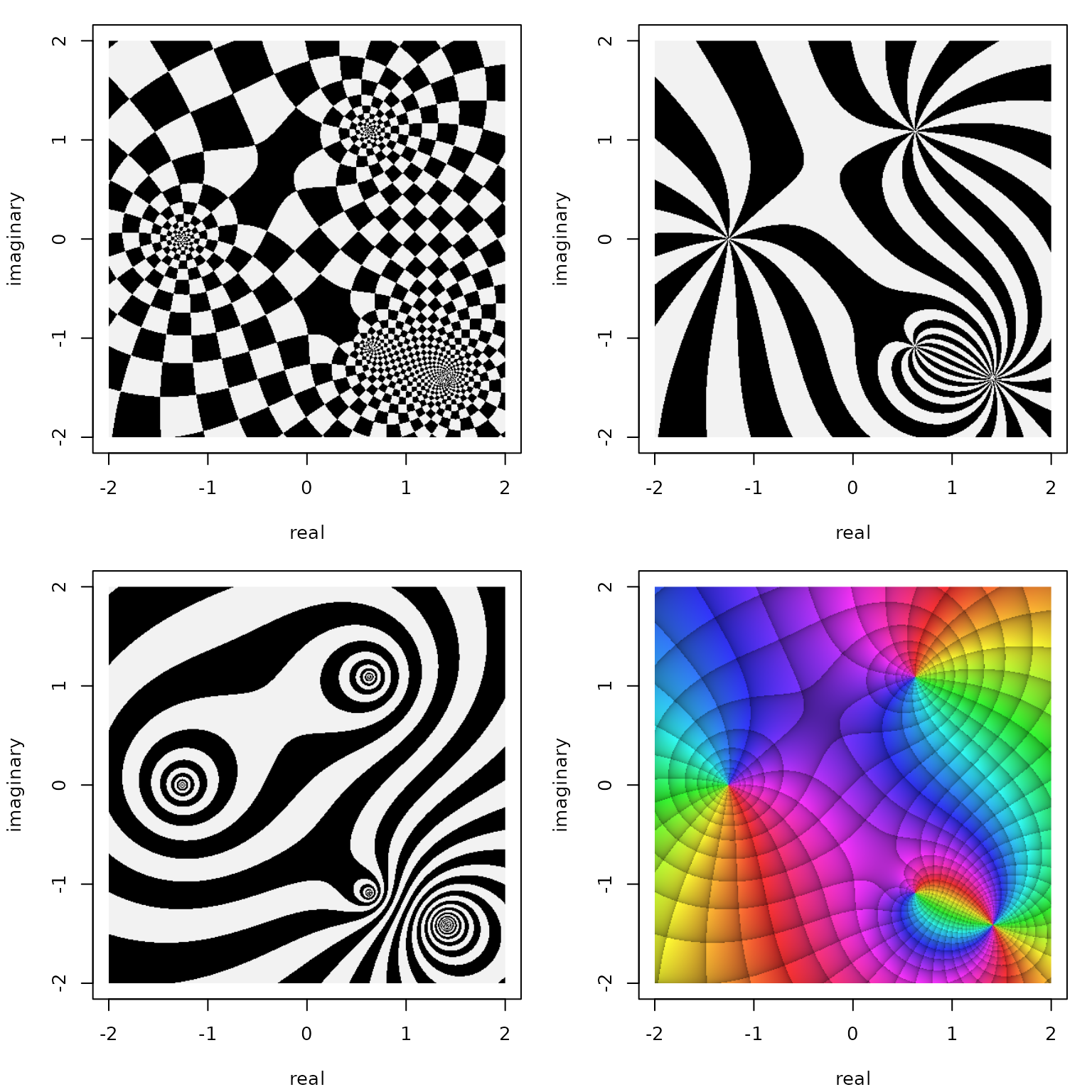

Two color portraits of the function \(f(z)=\frac{(z+\sqrt{2}\cdot\mathrm{i}-\sqrt{2})^2}{z^3 + 2}\) made with phasePortraitBw and byType ‘ma’ (top left), ‘a’ (top right), and ‘m’ (bottom left) together with a full phasePortrait (bottom right).

While the letters ‘Bw’ in phasePortraitBw stand for ‘black/white,’ the natural colors for such chessboard plots, the user is not limited to these. The choice of colors is defined by the parameter bwCols which, by default, is set as bwCols = c("black", "gray95", "gray"). The first and the second color are used for coloring the alternating zones, while the last color is used in cases where the function of interest produces results which cannot be sufficiently evaluated for modulus or argument (NaN, partly Inf). Note that the second color, "gray95" is almost, but not exactly white, which contrasts ‘white’ tiles against a white background in a visually unobtrusive way. The parameter bwCols can be freely changed; values must be either color names that R can interpret (call colors() for a list) or hexadecimal color strings like e.g. "#00FF32" (the format is "#RRGGBB" with ‘RR,’ ‘GG,’ and ‘BB’ representing red, green, and blue with an allowed value range of 00 to FF for each).

Aesthetic hints

While phase portraits were originally invented for scientific and technical purposes, their aesthetic quality is a feature in itself. In this section, we give a few technical hints that might be helpful for obtaining appealing graphics. We will be not only talking about features implemented in this package, but also mention some useful options provided by R base graphics. A general recommendation when plotting for maximum aesthetic results is also to first check out the function to be plotted with lower resolutions (e.g. the default 150 dpi), and a smaller format (but with the desired device aspect ratio), adjust the domain (xlim, ylim), and all other parameters of phasePortrait you might want to change (including the parameters gamma and stdSaturation we have not mentioned in this vignette, so far). Only if you are satisfied with the result at that stage, you should start the run with the desired final resolution and format, as plots at high resolution and large formats may be time-consuming depending on your hardware (see also the section defining image quality). When using the function riemannMask you could try changing the mask’s transparency (alphaMask) and it’s color (colMask). Often, black is a good alternative to the default white). Besides such simple issues there are, however, a few points we will talk about in more detail below.

The par(op) mechanism

As mentioned above, phasePortrait uses R’s base graphic system. This is a powerful tool, its functionality is, however, not always easy to understand and use. Many fundamental settings of base R graphics are stored in a set of parameters, which can be set or queried using the function par(). Among the important graphical parameters in our context are those which steer the outer margins and the plot margins (oma, omi, mar, mai) and those which define the default background and foreground colors (bg, fg). Type ?par to see a documentation of all parameters. Changing these parameters here and there during an R session can easily lead to graphical results that may be nice but hard to reproduce. For avoiding this, when par() is called to change one or more graphical parameters, it invisibly returns all parameters and their values before the change. These can be stored in a variable, and used to restore the original parameter values after the plotting has been done. This concept seems to be unknown to surprisingly many users of R:

# Set the plot margins at all four sides to 1/5 inch with mai,
# set the background color to black with bg, and the default foreground
# color with fg (e.g. for axes and boxes around plots, or the color of
# the circle outline from the function riemannMask).
# We catch the previous parameter values in a variable, I called
# "op" ("old parameters")
op <- par(mai = c(1/5, 1/5, 1/5, 1/5), bg = "black", fg = "white")

# Make any phase portraits and/or other graphics of your interest
# ...

# Set the graphical parameters back to the values previously stored in op
par(op)

Dealing with axes

Usually, when aiming for mainly aesthetic effects, you want to suppress plot axes from being drawn. As phase phasePortrait and phasePortraitBw accept, via the ... argument, all arguments also accepted by R’s plot.default, this can be easily achieved by providing the argument axes = FALSE:

phasePortrait("tan(z^3 + 1/2 - 2i)/(1 - 1i - z)", 
              xlim = c(-6, 6), ylim = c(-3, 3),
              axes = FALSE)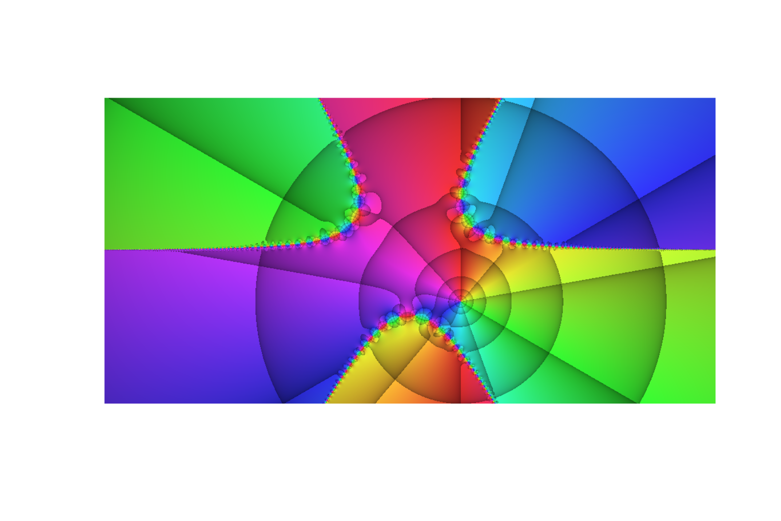

Phase portrait called with axes = FALSE. Note the unequal figure margins. These are R-default in order to reserve space for the usual annotations. Adjusting them is possible by means of the graphics parameters mar or mai as explained above.

This does, however, not only suppress both axes, but also the box usually drawn around a plot. If such a box is desired, it can be simply added afterwards by calling box():

phasePortrait("tan(z^3 + 1/2 - 2i)/(1 - 1i - z)", 
              xlim = c(-6, 6), ylim = c(-3, 3),
              axes = FALSE)
box()

If axes are desired together with a special aesthetic appeal (e.g. for presentations), it is worth trying out a black background and white axes. However, there are unexpected hurdles to take, before the result looks as it should:

# set background and foreground colors
op <- par(bg = "black", fg = "white")
# Setting the parameter fg has an effect on the box, the axes, and the axes' 
# ticks, but not on the axis annotations and axis labels.
# Also the color of the title (main) is not affected. 
# The colors of these elements have to be set manually and separately. While we
# could simply set them to "white", we set them, more flexibly, to the 
# current foreground color (par("fg")).
phasePortrait("tan(z^3 + 1/2 - 2i)/(2 - 1i - z)",
              xlim = c(-6, 6), ylim = c(-3, 3),            col.axis = par("fg"),
              xlab = "real", ylab = "imaginary",           col.lab  = par("fg"),
              main = "All annotation in foreground color", col.main = par("fg"),
              # Adjust text size
              cex.axis = 0.9, cex.lab = 0.9)
par(op)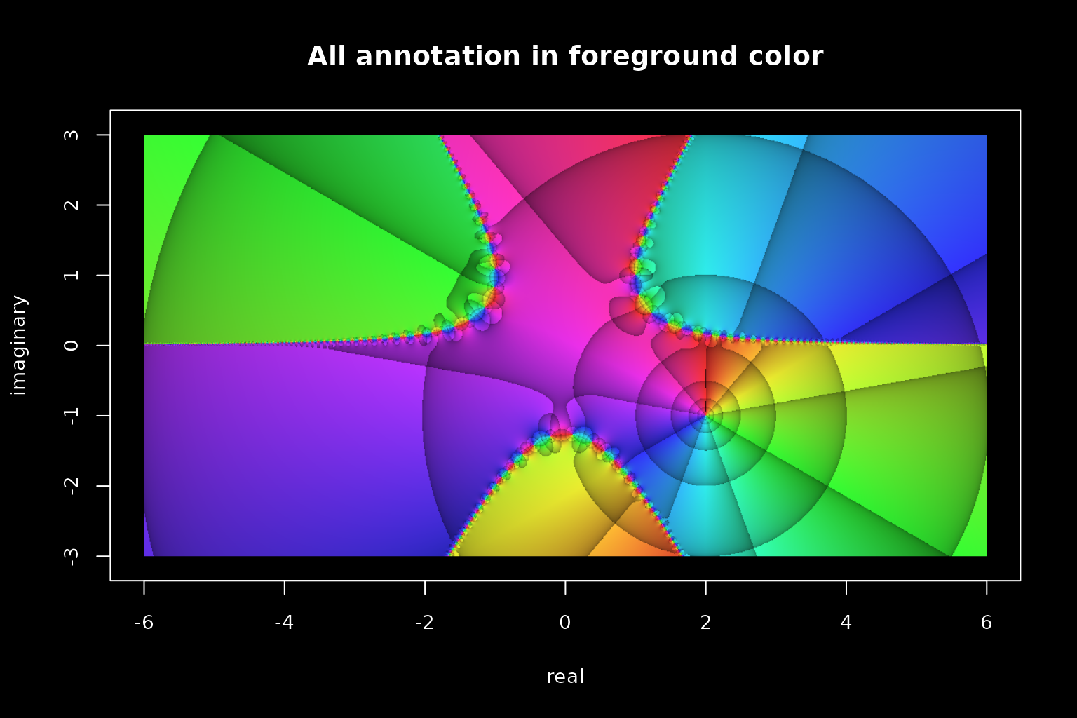

Note that by default the axes are constructed with an overhang of 4% beyond the ranges given with xlim and ylim at each end. More often than not this looks nice, but sometimes it is undesired, e.g. when a phase portrait is intended to cover the full display without any frame and margin. This behavior is due to the graphical parameters xaxs and yaxs (axis style) being set to ‘r’ (‘regular’) by default. Setting these parameters as xaxs = "i" and yaxs = "i" (‘internal’), no overhang is added. Both, xaxs and yaxs, can be either set in a call to par() or handed as arguments to phasePortrait. We will come back to these parameters in the following section.

Device ratio and margins

You might want to plot a phase portrait that fully covers the graphics device. The following code example shows how to achieve this. First, it is necessary to set the plot margins to zero (note that the outer margins are zero by default, so, usually, there is no need to care for them). Second, as phasePortrait uses an aspect ratio of 1 by default, xlim and ylim have to exactly match the aspect ratio of the graphics device to be plotted in. In order to facilitate this, we provide the functions ylimFromXlim and xlimFromYlim. In the example, we use the former in order to match xlim and ylim a device aspect ratio of 16/9. Third, in order to omit the 4% axis overhang (would look like a margin), the parameters xaxs and yaxs are set to “i.” Setting axes to FALSE is not absolutely necessary in this case, but is good style.

# Open graphics device with 16/9 aspect ratio and 7 inch width
x11(width = 8, height = 9/16 * 8)
op <- par(mar = c(0, 0, 0, 0)) # Set plot margins to zero
xlim <- c(-3, 3)
# Calculate ylim with desired center fitting the desired aspect ratio
ylim <- ylimFromXlim(xlim, centerY = 0, x_to_y = 16/9)
phasePortrait(jacobiTheta, moreArgs = list(tau = 1i/5 + 1/5), pType = "p", 
              xlim = xlim, ylim = ylim,
              xaxs = "i", yaxs = "i",
              axes = FALSE)
par(op)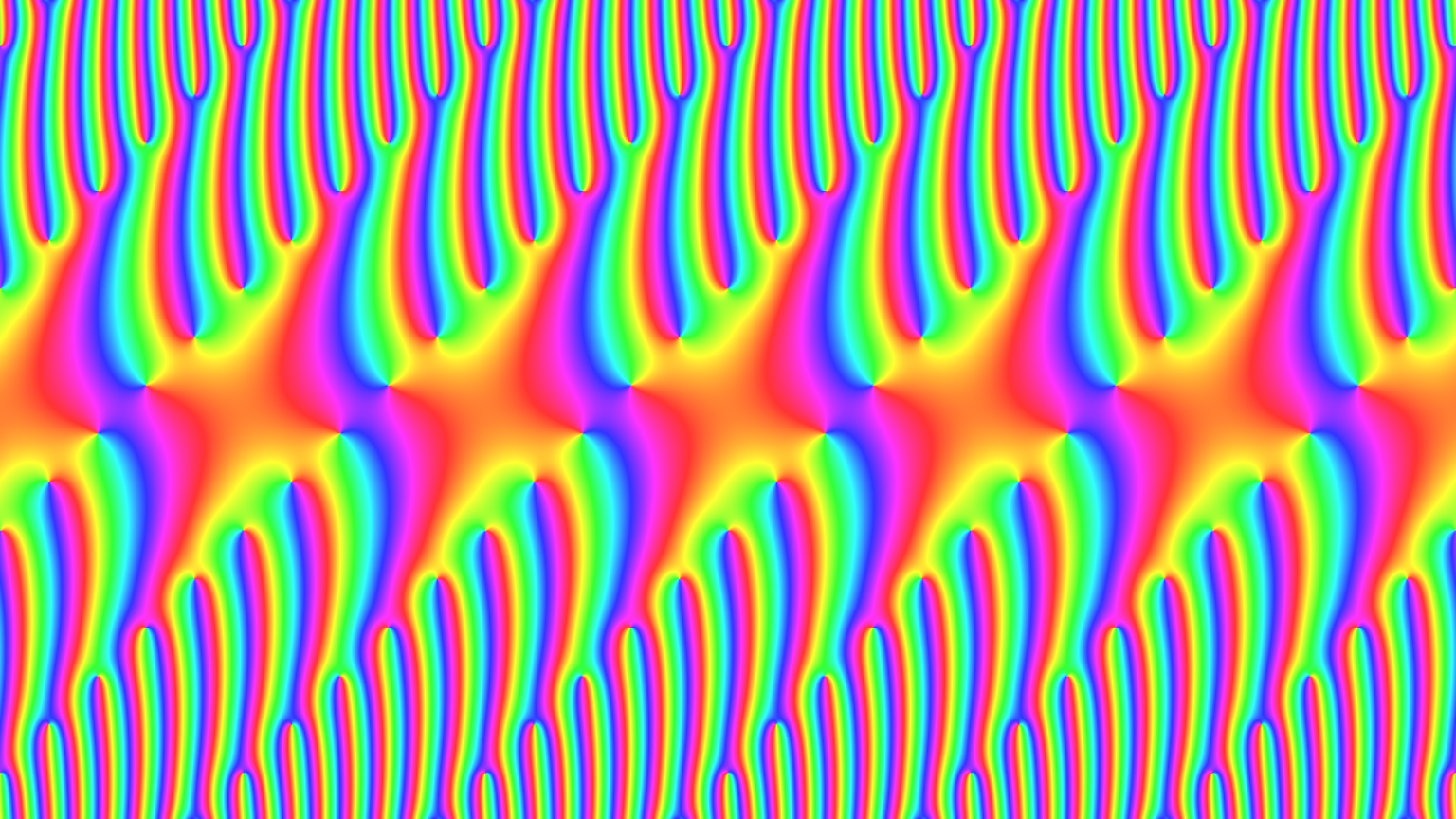

Not many changes are necessary for obtaining a phase portrait like above but with a frame. A convenient way to do this is to set the outer margins of the graphics device in inches with the graphical parameter omi and the background to the desired color. Adding this to the code above, however, leads to differing horizontal and vertical frame widths. This occurs because, due to the margin setting, the required ratio of the xlim and ylim ranges is no longer exactly 16/9. The precise ratio has to be calculated and provided to ylimFromXlim as shown in the code example below.

# Open graphics device with 16/9 aspect ratio and a width of 7 inches 
x11(width = 8, height = 9/16 * 8)
# Set plot margins to zero, outer margins to 1/7 inch,
#   and background color to black
outerMar <- 1/7 # outer margin width in inches
op <- par(mar = c(0, 0, 0, 0), omi = rep(outerMar, 4), bg = "black") 
xlim <- c(-1.5, 0.5)
# Calculate ylim with desired center fitting the desired aspect ratio;
#   however, the omi settings slightly change the required 
#   ratio of xlim and ylim
ratio <- (7 - 2*outerMar) / (7 * 9/16 - 2*outerMar)
ylim  <- ylimFromXlim(xlim, centerY = 0, x_to_y = ratio)
phasePortrait("sin(jacobiTheta(z, tau))/z", moreArgs = list(tau = 1i/5 + 1/5),
              pType = "p",
              xlim = xlim, ylim = ylim,
              xaxs = "i", yaxs = "i",
              axes = FALSE)
par(op)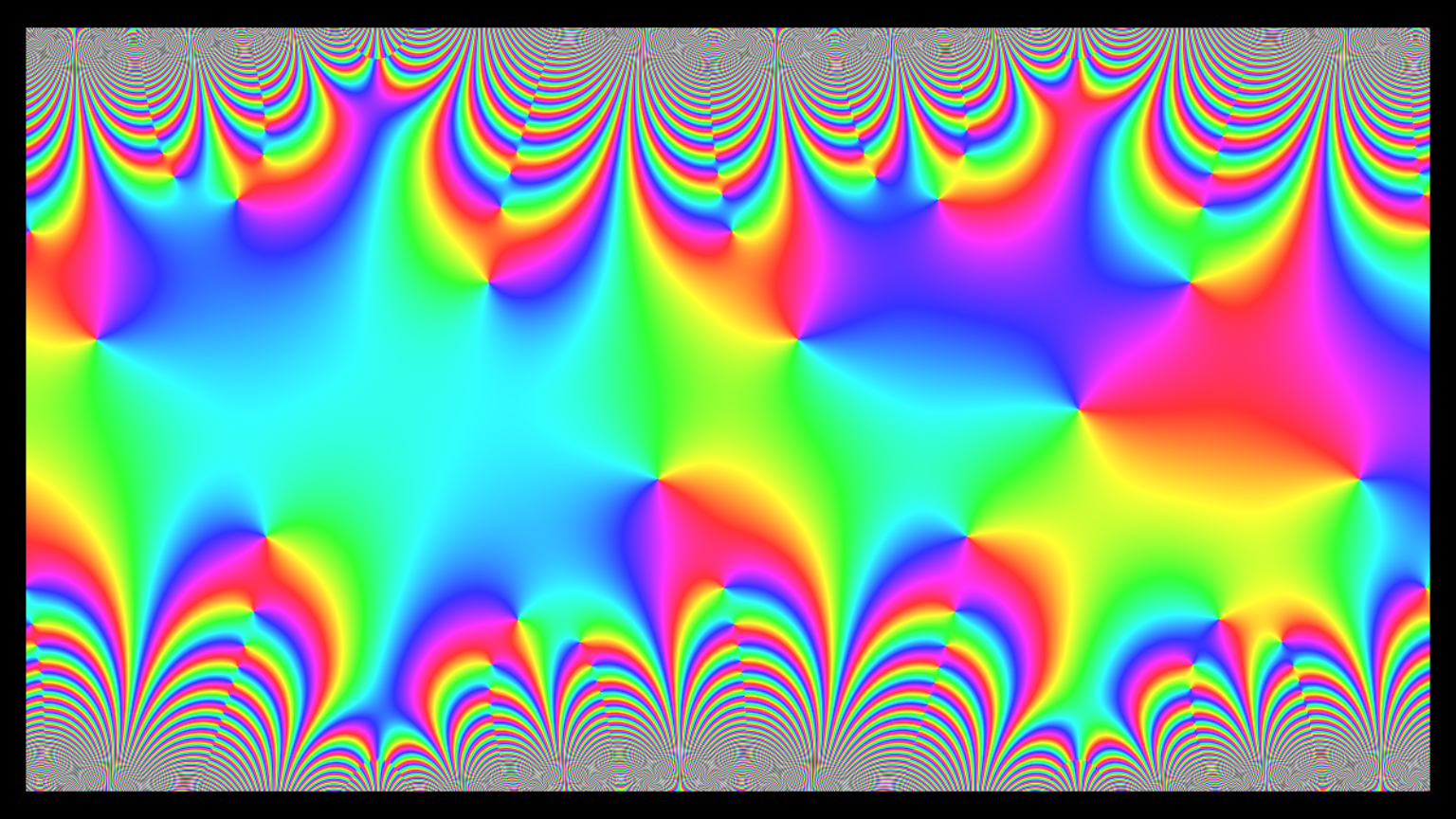

Technical moreabouts

This chapter details a few technical points which might be of interest for optimizing the results obtained by using the R package at hand. We talk about different ways to provide functions to phasePortrait, and about how to control image quality. And there is more: The function phasePortrait has to perform several memory and time critical operations. In order to keep memory utilization on a reasonable level and to optimize computing times, the function works with temporary files and parallel processing. We explain both below, because the user can influence their behavior. For avoiding unnecessary copying of big arrays, phasePortrait makes also use of pointers, but as there is no related control option for the user, we reserve this for a later version of this vignette.

Ways to provide functions to phasePortrait and phasePortraitBw

Quoted character strings

Any function to be visualized with phasePortrait or phasePortraitBw must be provided as the argument FUN. In some cases (see below), the argument moreArgs can turn out useful in combination with FUN. Probably the easiest way of defining FUN is a character string which is an expression R can evaluate as a function of a complex number \(z\). See some examples:

# Note that 'FUN =' is not required if the argument to FUN is handed to 
# phasePortrait in the first position
phasePortrait(FUN = "1/(1 - z^2)", xlim = c(-5, 5), ylim = c(-5, 5), nCores = 2)
phasePortrait("sin((z - 2)/(z + 2))", xlim = c(-5, 5), ylim = c(-5, 5), nCores = 2)
phasePortrait("tan(z)", xlim = c(-5, 5), ylim = c(-5, 5), nCores = 2)

If your expression requires arguments besides \(z\) you can provide them to phasePortrait by means of moreArgs, which expects a named list containing the additional arguments:

phasePortrait("-1 * sum(z^c(-k:k))", moreArgs = list(k = 11),
              xlim = c(-2, 2), ylim = c(-1.5, 1.5),
              pType = "p",
              nCores = 2) # Increase or leave out for higher performance 

While we recommend other solutions (see below), it is also possible to hand over more extensive user-defined functions as character strings. To make this work, however, the function must be wrapped in a vapply construct which guarantees the output of the function being a complex number by setting vapply’s argument FUN.VALUE as complex(1). Moreover, the first argument to vapply must be \(z\). In such cases, it is often convenient to define the character string outside the call to phasePortrait and hand it over after that, as we do in the following example:

funString <- "vapply(z, FUN = function(z) {
                  n <- 9
                  k <- z^(c(1:n))
                  rslt <- sum(sin(k))
                  return(rslt)
                },
                FUN.VALUE = complex(1))"
phasePortrait(funString, xlim = c(-2, 2), ylim = c(-2, 2), 
              nCores = 2) # Increase or leave out for higher performance

If such a function has arguments in addition to \(z\), they can be included into the call to ‘vapply’ and thus included into the string (for supporting this, we provide the function vector2string, see the example in its documentation), but we do not recommend that. Anyway, if you must know, here it is:

funString <- "vapply(z, FUN = function(z, fct) {
                  n <- 9
                  k <- z^(fct * c(1:n))
                  rslt <- sum(sin(k))
                  return(rslt)
                },
                fct = -1, 
                FUN.VALUE = complex(1))"
phasePortrait(funString, xlim = c(-2, 2), ylim = c(-2, 2),
              nCores = 2) # Increase or leave out for higher performance

Probably, the most useful application of this concept is when the vapply construct is pasted together at runtime with values for the additional arguments depending on what happened earlier. However, defining the function directly as a function first, and then simply passing its name to phasePortrait leads to a more readable code:

# Define function
tryThisOne <- function(z, fct, n) {
  k <- z^(fct * c(1:n))
  rslt <- prod(cos(k))
  return(rslt)
}

# Call function by its name only, provide additional arguments via "moreArgs"
phasePortrait("tryThisOne", moreArgs = list(fct = 1, n = 5),
  xlim = c(-2.5, 2.5), ylim = c(-2, 2),
  nCores = 2) # Increase or leave out for higher performance

As the function in the example above requires two additional arguments beside \(z\), we hand them over to phasePortrait via the argument moreArgs, which must be (even in case of only one additional argument) a named list (names must match the names of the required arguments), where the argument values are assigned.

Function objects

Besides character strings as shown above, the argument FUN can also directly take function objects. The simplest case is an anonymous function definition:

# Use argument "hsvNaN = c(0, 0, 0)" if you want the grey area black
phasePortrait(function(z) { 
    for(j in 1:20) {
      z <- z * sin(z) - 1 + 1/2i
    }
    return(z)
  },
  xlim = c(-3, 3), ylim = c(-2, 2),
  nCores = 2) # Increase or leave out for higher performance 

Evidently, this can be used with moreArgs as well:

# Use argument "hsvNaN = c(0, 0, 0)" if you want the grey area black
phasePortrait(function(z, n) { 
    for(j in 1:n) {
      z <- z * cos(z)
    }
    return(z)
  },
  moreArgs = list(n = 27),
  xlim = c(-3, 3), ylim = c(-2, 2),
  nCores = 2) # Increase or leave out for higher performance 

Any function object that is known by name to R, be it user-defined or contained in a package will work in the same way. Just hand over the function object itself:

# atan from package base
phasePortrait(atan, xlim = c(-pi, pi), ylim = c(-pi, pi),
              nCores = 2)

# gammaz from package pracma (the package must be installed on your machine
# if you want this example to be working)
phasePortrait(pracma::gammaz, xlim = c(-9, 9), ylim = c(-5, 5),
              nCores = 2)

# blaschkeProd from this package (moreArgs example)
#  make random vector of zeroes
n <- 12
a <- complex(modulus = runif(n), argument = 2 * pi * runif(n))
#  plot the actual phase portrait
phasePortrait(blaschkeProd, moreArgs = list(a = a), 
              xlim = c(-1.3, 1.3), ylim = c(-1.3, 1.3),
              nCores = 2)

# User function example
tryThisOneToo <- function(z, n, r) {
  for(j in 1:n) {
    z <- r * (z + z^2)
  } 
  return(z)
} 
# Use argument "hsvNaN = c(0, 0, 0)" if you want the gray areas black
phasePortrait(tryThisOneToo, moreArgs = list(n = 50, r = 1/2 - 1/2i),
              xlim = c(-3, 2), ylim = c(-2.5, 2.5),
              nCores = 2)

Defining own functions in C++ and using them with phasePortrait usually gives a substantial performance gain. This is especially true if they require operations that cannot be vectorized in R (i.e. if there is now way to avoid for-loops or similar). The ideal tool for integrating C++ code in R programs is Rcpp (Eddelbuettel and Balamuta 2017), but be aware that C++ functions compiled with Rcpp::sourceCpp will not work with phasePortrait, as this is not compatible with parallel processing. What it takes is to provide the C++ functions as or as part of an R package which is not difficult at all. The functions of the math family included in this package have all been coded in C++ and integrated with Rcpp.

Defining image quality

Clearly, there is a trade-off between the quality of an image plotted with phasePortrait and the computing time. The image quality is defined by the argument res and has a default value of 150 dpi. For pictures in standard sizes of about 30 x 20 cm plotting with 150 dpi does not take much time, and for many purposes, this resolution is sufficient. When resolutions of 300, 600 or more dpi are desired for high-quality printouts, we recommend to try out everything with 150 dpi (and, maybe, on a small format) before starting the final high-quality run. Technically, early after being called, phasePortrait gets the plot region size of the active graphics device and calculates the number of required pixels from this size and the value of res. Note, that R graphics devices for files, like png, bmp, jpeg and tiff, also expect a parameter res (if the units given for device height and width are cm or inches). For plotting to graphics files, we suggest to store the desired resolution in a variable first, and pass it to both, the graphics device and phasePortrait:

res <- 300 # Define desired resolution in dpi
png("Logistic_Function.png", width = 40, height = 40 * 3/4, 
    units = "cm", res = res)
phasePortrait("1/(1+exp(-z))", xlim = c(-25, 25), ylim = c(-15, 15), res = res,
              xlab = "real", ylab = "imaginary",
              nCores = 2) # Increase or leave out for higher performance
dev.off()

Temporary files

In order to keep the machine’s RAM workload manageable, phasePortrait will always save data in temporary files. These files are stored in the directory specified with the argument tempDir (default is the current R session’s temporary directory). After normal execution, these files will be automatically deleted, so, usually, there is no need to care about. Automatic deletion, however, will not happen, if the user calls phasePortrait with the parameter deleteTempFiles set to FALSE or if phasePortrait does not terminate properly. Thus, if phasePortrait crashed you should check the directory specified as tempDir and delete these files, because they usually are of considerable size. However, such orphans will never interfere with further runs of phasePortrait (see below).

The size of these temporary files depends from phasePortrait’s parameter blockSizePx (default: 2250000; it may be worth varying this value in order to obtain optimum performance on your machine). If the two-dimensional array of pixels to be plotted comprises more pixels than specified by this parameter, the array will be vertically split into blocks of that size. These sub-arrays are what is stored in the temporary files. More precisely, there are two temporary files per sub-array. One represents the cutout of the untransformed complex plane over which the function of interest is applied; the other contains the values obtained by applying the function to the first one. Thus, each array cell contains a double precision complex number; in a temporary file pair an array cell at the same position refers to the same pixel in the plot.

These files are .RData files, and their names adhere to a strict convention, see the following examples:

0001zmat2238046385.RData

0001wmat2238046385.RData

These are examples of names of a pair of temporary files belonging to the same block (sub-array). The names are equal except for one substring which can either be ‘zmat’ or ‘wmat.’ The former file contains an untransformed cutout of the complex plane, and the latter the corresponding values obtained from the function of interest as explained above.

Both names begin with ‘0001,’ indicating that the array’s top line is the first line of the whole pixel array to be covered by the phasePortrait. The name of the file that contains the subsequent array can e.g. begin with a number like ‘0470,’ indicating that its first line is line number 470 of the whole array. The number of digits for these line numbers is not fixed. It is determined by the greatest number required. Numbers with less digits are zero-padded. The second part of the file name is either zmat or wmat (see above). The third part of the file names is a ten-digit integer. This is a random number which all temporary files stemming from the same call of phasePortrait have in common. This guarantees that no temporary files will be confounded in subsequent calls of phasePortrait, even if undeleted temporary files from previous runs are still present.

Parallel processing

For enhanced performance, phasePortrait (and in the same way phasePortraitBw) uses parallel processing as provided via the R packages doParallel (Microsoft and Weston 2019) and foreach (Microsoft and Weston 2020). The number of processor cores to be used can be set with the parameter nCores when calling phasePortrait. By default, one less than all available cores will be utilized. Clearly, setting nCores = 1 will result in sequential processing. When phasePortrait is called with ncores > 1, and no parallel backend is registered, one will be registered first. The same applies, when a parallel backend is already registered, but the user desires a different number of cores. This registering may take some time. Therefore, when it terminates, phasePortrait does not automatically de-register the parallel backend (and register a sequential backend again). This saves registering time in subsequent runs of phasePortrait with the same number of cores to be used. This default behavior - keeping parallel backends registered after termination - can be changed by setting the parameter autoDereg on TRUE (default is FALSE). Otherwise, phasePortrait, after completing the plot, prints a message that the current parallel backend can be manually de-registered with the command foreach::registerDoSEQ(). We recommend to do this after the last call to phasePortrait in an R session.

There are three occasions, when phasePortrait utilizes parallel processing: First, after determining the size and number range (in the complex plane) of the whole two dimensional array of pixels to be plotted, the sub-arrays (blocks) corresponding to the parameter value blockSizePx are constructed and saved as temporary files in a parallel loop. These are the temporary files with the string zmat in their names (see section Temporary files). Second, while the single blocks are loaded and processed sequentially, each block is evaluated in a separate parallel process. In order to do so, the block is split into a few approximately equally sized parts; the number of these parts corresponds to the number of processor cores to be used. In each parallel process the function to be plotted is applied to each single cell of the corresponding block part (internally vectorized with vapply). The outcomes of all parallel processes are combined into one array which is saved as a temporary file which has the string wmat in its name. Third, for transforming the function values stored in the wmat files into hsv colors, a similar concept as in the second step is utilized: The single wmat files are processed sequentially, but the array stored in each file is split into chunks which are dealt with parallely. Eventually, transforming all wmat arrays results in one large color value array which can be plotted after that. Handling this large array is the most memory-intensive task when running phasePortrait, and it can take considerable time for large plots in high quality. So far, however, no alternative solution provided fully satisfying results.

As mentioned in the section about temporary files, users can possibly optimize performance by trying different values for the parameter blockSizePx. We mention this here as well, as blockSizePx does not only influence size and number of the temporary files, but also the size of the array chunks that are processed parallely.

Obviously, applying the function of interest to millions of values is time-critical. Therefore, when defining a function for a phase portrait in R, use all options at hand for vectorizing calculations. Moreover, you can count on a significant performance gain when you write time critical functions in C++. Thanks to the package Rcpp (Eddelbuettel and Balamuta 2017) this not really a hurdle anymore. As mentioned above, however, C++ functions compiled with Rcpp::sourceCpp will not work with phasePortrait, as this is not compatible with parallel processing; you have to provide such functions in a package. The package at hand provides a few functions (function family maths); all of them have been implemented in C++.

Acknowledgments

While this package is a leisure project, it would have been a mission impossible without the background of my daily work with R as a Forest Scientist at the Technical University of Munich (TUM). Fortunately, I have a job that allows me to learn about Nature by asking her questions (or trying to simulate what she is doing) with ever-improving methods and tools. I would like to thank everyone at the Chair of Forest Growth and Yield Science at TUM who keep me involved in discussions like: How can this be solved in R …

switch(1 + trunc(runif(1, 0, 6)),
       "... at all?",
       "... in a quick-and-dirty way?",
       "... in Hadley-Wickham-style?",
       "... without a loop?",
       "... without nested loops?",
       "... in a way somebody can understand?")

Veronika Biber provided expert advice for improving the vignette. Johannes Biber turned out the most patient pre-release tester one can imagine, boosting things with his high-end gaming machine. Thanks, guys! Also thanks to Gregor Seyer for his helpful review of the CRAN submission.

Clearly, programming in R would not be what it is, weren’t there some R titans who generously share their knowledge online. While I keep learning from all of them, I would like to thank especially Hadley Wickham and Dirk Eddelbüttel.

References

Eddelbuettel, Dirk, and James Joseph Balamuta. 2017. “Extending r with c++: A Brief Introduction to Rcpp.” PeerJ Preprints 5 (August): e3188v1. https://doi.org/10.7287/peerj.preprints.3188v1.

Microsoft, and Steve Weston. 2019. doParallel: Foreach Parallel Adaptor for the ’Parallel’ Package. https://CRAN.R-project.org/package=doParallel.

———. 2020. Foreach: Provides Foreach Looping Construct. https://CRAN.R-project.org/package=foreach.

Wegert, Elias. 2012. Visual Complex Functions. An Introduction with Phase Portraits. Basel Heidelberg New York Dordrecht London: Springer.